A couple of weeks ago, I said that I would document (at least for Jean S and UC) an observation about the use of squared weights in MBH98. I realize that most readers won’t be fascinated with this particular exposition, but indulge us a little since this sort of entry is actually a very useful of diarizing results. It also shows the inaccuracy of verbal presentation – which is hard enough even for careful writers.
MBH98 did not mention any weighting of proxies anywhere in the description of methodology. Scott Rutherford sent me a list of 112 weights in the original email, so I’ve been aware of the use of weights for the proxies right from the start. Weights are shown in the proxy lists in the Corrigendum SI (see for example here for AD1400) and these match the weights provided by Rutherford in this period. While weights are indicated in these proxy lists, the Corrigendum itself did not mention the use of weights nor is their use mentioned in any methodological description in the Corrigendum SI.
In one place, Wahl and Ammann 2007 say that the weights don’t “matter”, but this is contradicted elsewhere. For example, all parties recognize that different results occur depending on whether 2 or 5 PCs from the NOAMER network are used together with the other 20 proxies in the AD1400 network (22 or 25 total series in the regression network). Leaving aside the issue of whether one choice or another is “right”, we note for now that both alternatives can be represented merely through the use of weights of (1,1,0,0,0) in the one case and (1,1,1,1,1) in the other case – if the proxies were weighted uniformly. If the PC proxies were weighted according to their eigenvalue proportion – a plausible alternative, then the weight on the 4th PC in a centered calculation would decline, assuming that the weight for the total network were held constant – again a plausible alternative.
But before evaluating these issues, one needs to examine exactly how weights in MBH are assigned. Again Wahl and Ammann are no help as they ignore the entire matter. At this point, I don’t know how the original weights were assigned. There appears to be some effort to downweight nearby and related series. For example, in the AD1400 list, the three nearby Southeast US precipitation reconstructions are assigned weights of 0.33, while Tornetrask and Polar Urals are assigned weights of 1. Each of 4 series from Quelccaya are assigned weights of 0.5 while a Greenland dO18 series is assigned a weight of 0.5. The largest weight is assigned to Yakutia. We’ve discussed this interesting series elsewhere in connection with Juckes. It was updated under the alter ego “Indigirka River” and the update has very pronounced MWP. Juckes had a very lame excuse for not using the updated version. Inclusion of the update would have a large impact on a re-stated MBH99 using the same proxies.
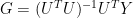
Aside from how the weights were assigned, the impact of the assigned weights on the proxies in MBH formalism differs substantially from an intuitive implementation of the stated methodology. In our implementation of MBH (and Wahl and Ammann did it identically), following the MBH description, we calculated a matrix of calibration coefficients by a series of multiple regressions of the proxies Y against a network U of temperature PCs in the calibration period (in AD1400 and AD1000, this is just the temperature PC1.) This can be represented as follows:
Then the unrescaled network of reconstructed RPCs 

However, this is Mann and things are never as “simple” as this. In the discussion below, I’ve first transliterated the Fortran code provided in response to the House Energy and Commerce Committee (located here ) into a sort of pseudo-code in which the blizzard of pointless code managing subscripts in Fortran is reduced to matrix operations, first using the native nomenclature and then showing the simplified matrix derivations.
You can find the relevant section of code by using the word “resolution” to scroll down the code, the relevant section commencing with:
c NOW WE TRAIN THE p PROXY RECORDS AGAINST THE FIRST
c neofs ANNUAL/SEASONAL RESOLUTION INSTRUMENTAL pcs
Calibration
Scrolling down a bit further, the calculation of the calibration coefficients is done through SVD operations that are actually algebraically identical to pseudoinverse operations more familiar in regressions. Comments to these calculations mention weights several times:
c set specified weights on data
…
c downweight proxy weights to adjust for size
c of proxy vs. instrumental samples
…
c weights on PCs are proportional to their singular values
Here is my transliteration of the code for the calculation of the calibration coefficients:
S0< -S[1:ipc]
# S is diagonal of eigenvalues from temperature SVD;
# ipc number of retained target PCs
weight0<- S0/sum(S0) #
B0<-aprox * diag(weightprx)
# aprox is the matrix of proxies standardized on 1902-1980
#weightprx is vector of weights assigned to each proxy;
AA<-anew * diag(weight0)
# this step weights the temperature PCs by normalized eigenvalues
[UU,SS,VV] <-svd(AA)
# SVD of weighted temperature PCs : Mann's regression technique
work0<- diag(1/SS) * t(UU) * B0[cal,]
# this corresponds algebraically to part of pseudoinverse used in regression
#cal here denotes an index for the calibration period 1902-1980
x0<- VV * work0
# this finishes the calculation of the regression coefficients
beta<-x0
#beta is the matrix of regression coefficients, then used for estimation of RPCs
Summarizing this verbose code:
[UU,SS,VV] < -svd(anew[1:79,1:ipc] * diag(weight0) )
beta= VV* diag(1/SS) * t(UU) * aprox[index,] * diag(weightprx)
Commentary: Mann uses SVD to carry out matrix inversions. There is an identity relating the pseudoinverse used in regression calculations to Mann’s SVD methods, that is very useful in analyzing this code. If the SVD of a matrix is represented as 
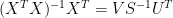
This can be seen merely by substituting in the pseudoinverse and cancelling.
Note that U,S and V as used here are merely local SVD decompositions and do not pertain to the “global” uses of U, S and V in the article, which I’ve reserved the products of the original SVD decomposition of the gridcell temperature network 
![[U,S,V]= svd(T,nu=16,nv=16)](https://s0.wp.com/latex.php?latex=%5BU%2CS%2CV%5D%3D+svd%28T%2Cnu%3D16%2Cnv%3D16%29++&bg=ffffff&fg=000&s=0&c=20201002)
Defining L as the k=ipc truncated and normalized eigenvalue matrix and keeping in mind that 
![[UU,SS,VV]= svd(UL,nu=ipc,nv=ipc)](https://s0.wp.com/latex.php?latex=%5BUU%2CSS%2CVV%5D%3D+svd%28UL%2Cnu%3Dipc%2Cnv%3Dipc%29++&bg=ffffff&fg=000&s=0&c=20201002)

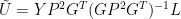
Applying the pseudoinverse identity to 


In our emulations in 2005 (and also in the Wahl and Ammann 2007 emulation which I reconciled to ours almost immediately in May 2005), the matrix of calibration coefficients was calculated without weighting the target PCs and without weighting the proxies (in this step) as follows:

The two coefficient matrices are connected easily as follows:

The two weights have quite different effects in the calculation. The weights 

Following what seemed to be the most implausible interpretation of the sketchy description, we weighted the proxies in the estimation step; Wahl and Ammann dispensed with this procedure altogether, arguing that the reconstruction was “robust” to an “important” methodological “simplification” – the deletion of any attempt at weighting proxies (a point which disregards the issue of whether such weighting for geographical distribution or over-representation of one type or site has a logical purpose.)
Reconstruction
Scrolling down a bit further, one finds the reconstruction step in the code described as:
“DETERMINE THE RECONSTRUCTED FIELDS BY INVERTING THE TRANSFER FUNCTION”
Once again, here is a transliteration of the Fortran blizzard into matrix notation first following the native nomenclature of the code:
B0 = aprox * diag(weightprx)
#this repeats previous calculation: aprox is the proxy matrix, weightprx the weights
AA< -beta
# beta is carried forward from prior step
[UU,SS,VV] -svd(t(AA))
# again the regression is done by SVD, this time on the matrix of calibration coefficients
work0<- B0 * UU * diag( 1/SS)
work0 <-work0 * t(VV)
#this is regression carried out using the SVD equivalent to pseudoinverse
x0<- work0
#this is the matrix of reconstructed RPCs
Summarizing by collecting the terms:
[UU,SS,VV] = svd(beta) )
x0= aprox * diag(weightprx) * UU* diag( 1/SS) * t(VV)
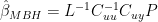
Commentary: Using our notation, the unrescaled reconstructed RPCs denoted by

Once again the pseudoinverse identity can be applied, this time for 


Expressed in terms of C matrices, this expression becomes:


The form of the above expression is precisely identical to the form of the expression resulting from application of the conventional expression for weighted regression shown above, which was (additionally incorporating the L weighting, which is removed in a later step):

However, there is one obvious difference. The Mannian implementation, which, rather than using any form of conventional regression software, using his ad hoc “proprietary” code, ends up with the proxy weights being squared.
In a follow-up post, I’ll show how the L weighting (but not the P weighting) falls out in re-scaling.
The Wahl and Ammann implementation omitted the weighting of proxies – something that they proclaimed as a “simplification of the method”. If you have highly uneven geographic distribution, it doesn’t seem like a bad idea to allow for that through some sort of stratification. For example, the MBH AD1400 network has 4 separate series from Quelccaya glacier (out of only 22 in the regression network) – the AD!000 network has all f in a network of only 14 proxies. These consist of dO18 values and accumulation values from 2 different cores. It doesn’t make any sense to think that all 4 proxies are separately recording information relevant to the reconstruction of multiple “climate fields” – so the averaging or weighting of series from the same site seems a prerequisite. Otherwise, why not have ring width measurements from individual trees? Some sort of averaging is implicitly done already. In another case, the AD1400 network has two ring width series from two nearby French sites and two nearby Morocco sites, which might easily have been averaged or even weighted through a PC network, as opposed to being used separately.
While some methodological interest attaches to these steps, in terms of actual impact on MBH, the only thing that “matters” is the weight on the bristlecones – one can upweight or downweight the various “other” series, but the MBH network is functionally equivalent to bristlecones +white noise, so upweighting or downweighting the white noise series doesn’t really “matter”


14 Comments
Well, to detect mathematical smoke screens , this is the only way to go. For example, Hadley says that
And then there’s no further explanation.. And code that generates s21 CIs is not available. I’ve seen this method applied elsewhere (non-climate science).
MBH9x algorithm is another smoke screen, the underlying model behind the smoke is
Y=XB+n
where Y is proxy record and X is matrix of annual grid-box temperature. Matrix B is not restricted in any way!
I’m having trouble parsing this sentence.
Should “falls” be outside the parentheses?
Is “our in” a transposition of “in our”?
Or is “our” a typo for “out” as in “falls out in”?
Steve: Yes. Corrected.
ve
Oh dear, something disastrous has happened to my intended posting. Seems to have vanished into the bowels of XPPro. I’ll have to re-write it all, but not now – too late for me to think straight. Sorry about that. The ve. is all that’s left :-((
I’ll take your word for the math, Steve, but I’m sure you’re correct.
However, the real problem I see with this aspect of the MBH procedure is not that they square their weights, but that they are using arbitrary weights. The square of an arbitrary weight is no more arbitrary than the original weight itself, so it is not clear that squaring these weights makes them any worse.
Your first and second equation do multivariate “Classical Calibration Estimation”, as discussed by UC in last year’s thread “UC on CCE” at http://www.climateaudit.org/?p=2445, based on an equation in the calibration period like
Y = UG + E,
where Y is an nxq matrix of proxies, U is an nxp matrix of temperature indicators or PCs, G is a pxq matrix of coefficients determined in your first equation, E is the nxq matrix of errors. (I’ve suppressed the constant term, but that should be in there as well.) Your second equation estimates a reconstructed value (or values) of U, say U*, from new values of the proxies, say Y*, under the assumption that the G’s are the same as in the calibration period.
However, the correct P matrix to use is not what feels good (per Mann), but rather the reciprocal of an estimator of the covariance matrix of the residuals. If p and q are small in comparison to n, and it looks like the variances are unequal and there are non-zero covariances, the obvious estimator of this covariance matrix is Ehat’Ehat/(n-p-1), using calibration period values of the residuals Ehat. If p and q are biggish relative to n, the method will still work, but perhaps only if you impose enough parsimonious restrictions on it. If you think the proxies should be independent (probably untrue for MBH), you can even make P diagonal.
In no event, however, do you determine weights, as Mann did, by just looking at the proxies in isolation rather than at the variances and covariances of their residuals in the calibration equations. Mann is evidently muddling together the variance (or standard deviation?) of the proxy itself with the variance (or standard deviation?) of its residuals in the calibration equation.
Incidentally, if the covariance matrix is diagonal, and one happens to know the inverse standard deviations of the errors rather than their inverse variances, then these weights should in fact be squared. I’m sure Mann just didn’t realize what he was doing, however.
Steve,
You may remember sending me the MBH98 data several years ago, I think as an Excel file, for which I’ve been eternally grateful! You also sent the weights used by Mann, and the identifications of the hitherto mysterious (scaled) temperature data cols 21 – 31.
I’ve worked in my somewhat simplistic fashion on this wealth of information for a large number of hours, and I hope that I’ve arrived at a reasonable understanding of what might be gleaned from it.
Reading your post above (which left my matrix algebra far behind I fear) I have been trying to get to grips with the concept of “calibration” in the context of the 112 columns. I always ask myself why it is necessary, and here you may well be able to sort me out. The view that I take is that Mann et al assembled, presumably in good faith, a large collection of data that they thought might be indicators of climate. The original values were from many sources, and amongst them was a formidable array of dendrochronological stuff. I wrote to Prof Mann, in the form of a handwritten airmail, which generated an immediate reply with references to sites where I could download large amounts of data – several hundred columns – which were I have presumed the data from which he formed his principal components as reported in the 112 published data columns.
As a total amateur I have no way in which I could assess the technical validity or otherwise of the columns labelled PC1, PC2 etc, but I have presumed that each of them represents something that a knowledgeable person would expect to be related systematically to the climate parameter that most of us believe to be of great significance on the worldwide scale, to wit temperature. It would be comfortable to be able to assume that such a relationship was roughly “linear”, and positively correlated with temperature, our target parameter. If it were not, why would anyone wish to include it in a rational assembly of climate indicators?
So, I begin with this assumption. Next, perusing Mann’s data one is instantly struck by the amazing variability in the scale and location of the recorded data. There is no way one could hope to build a meaningful composite value (some sort of average) from data on such diverse and seemingly random collection of numbers. Thus I took the rather obvious step of standardising each column to mean zero, variance one. Neglecting the now hot topic of column weights one can average across the data rows to form some sort of estimate of what the “climate” was like during any given year, on a standardised scale having no practical units attached to it. In order to relate this to some sort of real temperature scale one would have to have reliable actual temperatures values from some source. The stumbling block I have is that I cannot see where this information, which I think must necessarily come from outside the Mann data collection, arises. Where is it reported, and where can it be verified?
So there’s the fundamental problem I cannot resolve for myself.
In my investigations of MBH98 I have sidestepped (ignored) the calibration problem, and used simple averages across columns (or single columns) as an index of climate The 112 columns individually make for unwieldy handling and reporting, but it seems to me to be a logical step to assemble the standardised columns into “homogeneous” groups. For example, columns 1 – 9 are all from observations on tropical seas, 10, 11 and 21 – 31 are “real” temperatures – i.e. not proxies, although from various regions (weighted towards Europe) – but are presumably a potential source of a “gold standard” for calibration purposes. I selected 9 groups- someone else might well have chosen differently – and looked carefully at the behaviour of these over time. Of course the records are of varying length, but there is a core set starting in 1820 and ending around 1970 for which every column is complete.
If one is searching for confirmation of the alleged “hockey stick” property of Mann’s data set this time period is quite appropriate as a data base. Its centre is roughly the spot where the HS is said to become apparent. Some people might well propose using the correlation coefficient as a means for identifying, or even quantifying, a possible relationship between the various groups, but this is far too restrictive and prescriptive in my opinion. Remember that correlation coefficients are computed as /linear/ correlations, and totally ignore the most important property of these data, which is that they are time series, and thus have a considerable degree of inherent commonality. What we need is an objective method of comparison that uses this vital component of our information. Based on industrial experience in investigating the past behaviour of test rigs my obvious choice was to form the cumulative sum of the data over the period of interest using the period mean as the basis of the cusum. This is a very simple operation which anyone who has used a spreadsheet can readily program. I don’t use spreadsheets, but some statistical software that carries out this sort of operation in a very simple way.
One great property of cusum analysis lies in its remarkable ability to display the major features of a time series even in the presence of substantial amounts of “noise” – in this case the supposed random component of climate data. Another is the ease with which periods of stability can be identified, and because of this the ease of detection of rapid or abrupt changes in regime.
Having identified possible periods of stability it is easy to examine these by standard statistical methods – trend analysis for example – to confirm of refute the indications provided by the cusum plot. The general grand scale form of the cusum indicates the overall trend in the data, which for climate data over the last 100 to 200 years is upwards as we know. This results in a roughly U or V shaped cusum plot, but with very important details. These are the aforesaid periods of stability, characterised by roughly straight segments of the cusum, and periods of rapid, detectable, change, indicated by a clear curved cusum segment. Changes may be steady or in the case of single site data very abrupt indeed. To verify this look at data for NW Atlantic (Greenland) sites for the last 100 years and concentrate on what happened near September 1922. There is loads of data available, including some very recent and brilliantly assembled stuff by Vinther et al.
Looking at MBH98 it is very apparent that the real temperatures and most of the proxies produce related cusum patterns. This is rather encouraging, I think, but what is NOT shown on these cusum plots is anything remotely indicating the cusum of a hockey stick.
If anyone reading this would like to see some plots I shall be delighted to provide some from my huge archive! Can’t do that in this posting because I use two totally different computer systems which cannot as yet be linked readily. However, I can do it in a two stage operation, and anyway I’ve not yet found out how to post them to a forum such as this :-((
You really have to see these plots, of which I have many hundreds!, to appreciate properly what can be found using industrial engineering technology on climate data.
I have loads more to write should anyone be interested.
Please respond, or shoot me down if you wish!
Robin
Re #5
Robin,
You said:
“Thus I took the rather obvious step of standardising each column to mean zero, variance one. Neglecting the now hot topic of column weights one can average across the data rows to form some sort of estimate of what the “climate” was like during any given year, on a standardised scale having no practical units attached to it.’
I assume that you averaged the rows of deviations of the normalized column data. If so, it seems to me that is ok if the data in the columns are normaly distributed and stationary. If the column data are not normally distributed or stationary, the row average is the row average but may be meanningless. For example, if you normalize such a row average, the cumsum plot may show well-defined trends that cannot be explained.
I have used your method when trying to understand local and regional temporal and spatial variations in USHCN surface temperature data. The U’s and V”s are eye-appealing but the underlying non-linearities and non-stationarity are confounding.
I have a somewhat shorter question for Steve, namely after MBH have estimated the temperature PC’s U as in your second equation, how do they get from there to NH temperature T? This never seems to be discussed, and MBH 9x don’t offer much help. Is there a second CCE exercise where the U’s are calibrated to T, or are the U’s just averaged together somehow?
Is there really any point in bothering with the temperature PC’s if one is ultimately only interested in T? Just calibrating T directly to the Y’s would be a lot simpler.
Mann’s smoke screen is quite efficient, I’m about to get lost 😉 Anyway, Hu in #4 links to my post that begins with residuals My_recon – original_MBH99, and I get this match without these scaling steps (P,L) (hence I write about identity S in my post, S^-1 = P in Steve’s notation). Some notes:
1) My code downloads temperature U-vectors directly, I’ve tried to reproduce them via SVD, monthly gridded temperature data needs to be multiplied by cosine lat gridponts.tx and divided by tcpa-standard.txt and then SVD and then downsampled to annual to get quite close to archived U-vectors.
2) I don’t use P or L, but if I undestood correctly, L cancels out. So the remaining difference between my and Steve’s implementation is P. And as Hu notes, P (S^-1 in my post) by Mann is not obtained in conventional way, I tried conventional P in my post, http://signals.auditblogs.com/files/2007/11/ad1600_rec_cce.png
In #6, HMcCard asked for a bit of clarification of the method I used in examining MBH98 data.
The reason for standardising each of the data columns was to avoid spurious weighting that would occur if the “raw” values, as published by Mann et al were used. The shape of the plots of individual columns against the time variable is of course totally unaffected by this transform. Its departure from the mean of column time series is simply a measure of how each column value differed from its mean, and thus I think it is reasonable to average across column to provide an estimate of the consensus value of the departure from the mean for the data as a whole (or as a rational sub-sample) of the data columns for each data year. After all, it must be supposed that in any given year each data column would be reflecting the climate of the time, otherwise why bother with time series at all.
Using a restricted data set, the period from 1820 to 1980, all columns are complete with what one hopes are valid observational numbers. The standardisation is thus unlikely, I feel, to produce a biased mean.
Of course, the data in the columns are /NOT/ stationary! They are climate data, and thus change due to a variety of factors, and without doubt the general change over this period has been upwards. That is what we are interested in, I think, and what I hope to do is to demonstrate the manner in which this upward trend takes (took) place. What I find is that much of the change took place over restricted periods of time, with generally stable periods between the change events or segments. Individual data columns also show this type of behaviour, and it is really interesting to look at the form of the cusums of the single columns. Some appear to be genuine un-tampered with data, but others show very strong signs of having been smoothed before being reported. Cusum plots demonstrate this very easily. For single site data, or assemblies of data of very similar origin such as the 13 temperature columns, transitions between stable regimes are generally very clear indeed, thus encouraging me to believe that the cusum method holds some promise in evaluation of assemblies of time series data.
If someone can tell me how to insert a GIF into this contribution (presuming it’s allowed) I’ll be very happy to show just what happens using these techniques.
It is very interesting to read that you have also used a technique similar to mine. I wonder exactly how you interpret the cusum patterns. I contemplate the very grand scale shape, and propose an hypothesis – “the region between 1830 and 1854 is stationary” for example – and then test the original data to see if this hypothesis holds up. Another hypothesis might be “In late 1922 a very abrupt change took place”. This would be signalled by something approaching an elbow in the cusum plot. It could be verified by a higher resolution analysis, using monthly rather than annual data, suitably de-seasonailised, and by examination of the apparently more stable segments on either side of the hypothesised elbow. Such “verification” of the import of cusum plots seems to work very well.
I certainly am not a fan of hypothesising a simple linear model to climate data and working with the residuals. This seems to be a standard technique for inducing stationarity over a chosen period, but my knowledge of standard time series methods is slight. As for assessing the data for having a normal distribution I really cannot be sure of how this might affect ones deductions if it were found not to be the case. In my experience attempting to disprove the hypothesis that a given collection of observed data are normally distributed is seldom successful, unless is is grossly and obviously non-normal, such as daily temperatures over a year in a non-tropical site. How would non-normality influence deductions regarding climate data. I’ve nothing to base any ideas on, so would welcome some instruction.
Robin
Robin, you need to have a website somewhere you can upload your images to, and link from there – if you do not have server space, there are free accounts you can set up such as photobucket.com or imageshack.com that allow you to upload images.
Having uploaded your image somewhere, copy ONLY the direct URL of the image to your clipboard (i.e. without any enclosing BB or HTML code), click the [ Img ] button above the comment box and paste your URL in.
The image may not show in the Preview (that’s a software bug), but should be displayed when you submit the comment. A direct URL pasted in your comment may be a useful back up until you get used to how everything works.
Robin,
Re #9
Robin,
I’ll try to be brief in my response to your request but I may be sniped for being off-topic. If so, contact me and we can continue the dialogue via e-mail.
As we both know, your so-called CUMSUM method is a simple way to find data trends and evaluate trend patterns. Permit me define a few terms that I will use; you might have something else in mind for the same term. First, I’m referring to an nxm data array where the data observations and index to n-rows in m-columns. The data in each column is normalized by transforming the raw data point in each cell to become the difference between the data point and the column average (or arithmetic mean) divided by the STDEV of the column data. The data normalized data in each cell is measured in STDEV units. After normalizing each data column, a new nxm array can be formed for the normalized data set. Of course, the normalized data in each column can be integrated to form a CUMSUM column to look temporal changes in the form of trends. Second, I am referring to persistent trends wherein the deviations in several adjacent cells either are more or less than the column average. For example, if the row index is in years, decadal trends would be persistent. Third, graphical display of single CUMSUM data column may show easily-recognized V- and U-shaped trends and/or invert V- and U-shaped trends. The V-shaped trends may be the most interesting and perplexing because it signifies an abrupt or stepwise change in the underlying data has occurred that changed the sign of the slope of the CUMSUM curve. Of course, a U- shaped trend is a steep negative slope followed by a near-zero slope followed by a steep positive slope. A quadratic-shaped or conic section-shaped trend is also common and easily recognized. It is caused by a linear trend in the underlying data where curvature of the CUMSUM trend depends on the slope of the linear trend in the underlying data. If the CUMSUM trends for each column are significantly different in shape and phasing from other columns, different factors are influencing the underlying data. Finally, I am referring to stationary as being the stability of the statistical distribution of the data in a column. I am not referring to the stability of a trend. The data in a column doesn’t have to normally-distributed to be stationary. In long data columns, it is quite possible the data are normally-distributed over a long string of cells but become skewed or non-normal in other strings of cells. These changes in distribution mean the data are non-stationary.
As I mentioned in #6, I was trying to understand the temporal and spatial variations in some USHCN surface temperature data. I chose several sites where monthly data was available from 1897 to 2005. Hence, my data array was 109×12 for each station. After normalizing the monthly temperature data in each column, I plotted the CUMCUM data. As you know, all CUMSUM data columns start at zero and return to zero. The difference in the trajectory of the CUMSUM curve over the 109 cells in a monthly column sets the trend pattern. I was struck by the differences in the trend patterns for each month. Although some monthly patterns were similar in some features, there were many significant differences. For example, at one site, there essentially no persistent trends in November over the 109 yr interval whereas large decadal trends were observed in the trend patterns for October and December. I observed the same perplexing similarities and differences in trend patterns for the other sites that I examined.
I’ll not take the time to describe the similarities and differences. Suffice to say, they involved V-, U-, conic-shaped trends and phase delays, as well as, non-normal and non-stationary inter val. All of this indicated there were many other inexplicable non-linear factors influencing the temperature data. Some of the factors were undoubtedly due to weather matters and other related to longer-term climate changes.
Yes, it is possible to add another column in the data array and include the average of the 12 monthly data column. The CUMSUM for the average annual data exhibits its own trend pattern and it is different from any of the monthly patterns. That’s no surprise since averaging step is merely the equal weighting or blending of the monthly data. This obviously suppresses or obscures all but the large amplitude trends. In #5, I understand that you averaged your 112 column data set (not the normalized data set) to from an equally-weighted “total” data column. If my understanding is correct, then I believe that most of the lesser trends are suppressed. Therefore, this is different than using a PC methodology to select a smaller number of unequally-weighted data columns.
So … this probably didn’t provide you with any new insights. My cautionary note would be: “ … be sure that you have an idea about what kind of trends that you are looking for before using too highly aggregated data sets.”
Hu,
Reconstructed Us are multiplied by original S and V^T, and then re-scaled by tcpa-standard.txt , and this is the grid-point reconstruction. RE’s and other stats are computed from cosine-weighted averages of this grid-point recon (NH, sparse, global etc.). This is, of course, wrong way to compute these stats.
I’m still puzzled by P-weights, without these weights I can replicate MBH99 results more accurately..
#12. UC, It’s possible that he didn’t use P-weights in MBH99, just in 98. I’ll experiment a little with that. There are some odd changes between the two studies – the secret CI method in MBH99 is still puzzling. Also he used 3 NOAMER PCs in AD1000 as opposed 2 NOAMER PCs in 1400 and 1450 – something that would seem impossible if he used a Preisendofer-style Rule N, as he said .
Steve,
I use http://www.nature.com/nature/journal/v430/n6995/extref/FigureData/nhmean.txt and http://holocene.meteo.psu.edu/shared/research/ONLINE-PREPRINTS/Millennium/DATA/RECONS/nhem-recon.dat
no differences in NH mean, and without P I can replicate that better. Yet, there is another version of MBH98 somewhere, see http://www.ncdc.noaa.gov/paleo/ei/ei_attriold.html
One Trackback
[…] serious problems with their use (or non-use) of the covariance matrix of the residuals. See, eg, “Squared Weights in MBH98″> and “An Example of MBH […]