Chas. has sent in a recipe for showing random walks in Excel. These sorts of things are much, much easier in R (see http://www.r-project.org for free download). I’ve posted up a little script below which generates random walks and ARMA(1,1) walks together with trend lines and t-statistics.
The generating script shows (1) random walks with steps ("innovations") distributed from a normal distribution; (2) ARMA(ar1=0.92,ma1= -0.32) walks with innovations distributed from a normal distribution with standard deviation =0.2. These parameters can be easily changed. The examples have N=321 (the length of the current satellite record.) In each case, the script shows the trend line, the slope coefficient and the OLS t-statistic (usual significance 1.96).
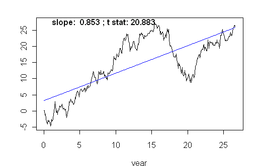
If you plot a few examples, you will see that a trend fitted to a random walk generates a "significant" trend nearly all the time for a series of length 321. The random walk is obviously "more explosive" than an i.i.d. series, as illustrated at realclimate. A random walk as shown here has an AR1 coefficient of 1 and MA1 coefficient of 0.

Figure 1. Example of random walk with trend line.
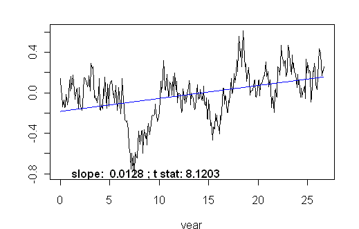
ARMA coefficients that more reasonably mimic the behavior are ARMA (ar=0.92; ma= -0.32). This type of "random walk" does not generate "significant" trends nearly as often as a random walk with ar =1. However, this process generates a lot of "significant" trends. The figure below (with a trend of 0.020 "degrees C/decade") was the 5th one that I generated. Obviously, the "look" of series generated with these parameters has a similar "look" to the actual satellite series, while i.i.d series (or random walks for that matter) do not.

Figure 2. Example of ARMA (ar=0.92, ma= -0.32) walk with innovation sd = 0.11. Seventh draw.
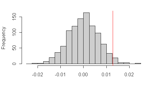
John Hunter has posted up some examples arguing the merits of OLS trend statistics. My take on the difference in approaches is that my concern is directed towards false positives, while John’s is directed towards false negatives. Both are valid issues. I think that the resolution of the points of view comes through accurately describing "confidence intervals" . I’ll come back to some of these issues later. Without commenting in detail on these examples, for now, I’d like to present some simulation data from ARMA (ar=0.92, ma= -0.32, innovation sd=0.11) walks as generated above (1000 examples). I fitted an OLS trend to each one. Figure 3 below shows the distribution of slope coefficients. The OLS trend of the satellite series (0.0128 deg/year) is at the 97th percentile for draws generated from 0 trend. This graphic also provides information on likelihoods with other trends. For example, let’s suppose that the "true" trend was 0.05 deg C/decade rather than 0 deg/decade: this would shove the graphic to the right with respect to the red line and make it about the 64th percentile with a lower "true trend". (Equally the observations could result from an ARMA(1,1) process with a larger trend than the OLS trend.

Figure 3. Histogram of 1000 slope coefficients from ARMA (1,1) simulations with satellite-like coefficients.
What the simulations indicate is a very wide range of slope coefficients generated from a similar process. The problem of "spurious significance" is that the OLS t-statistic becomes very unreliable – this is what "spurious significance" means: not that the trend is or isn’t "significant", but that the statistic purporting to indicate "confidence" in the trend isn’t significant. Here is a histogram of the t-statistics from the above regressions fitting a line to the realizations, with the red lines showing the usual "95% significant" levels of 1.96. In fact, "spurious significance" is shown 68% of the time with a conventional t-statistic. For 95% significance, the t-statistic needs to be about 9.28.

Figure 4. Histogram of t-statistics. Red lines show usual OLS 95% significance level.
Granger and Newbold[1974] was written in 1974 and has spawned much work which I’ve promised to discuss and gradually am getting to. One of the main strategies for analyzing spurious relationships is focusing on benchmarks for the t-statistics, so that they more appropriately emulate the properties of the process being modeled. I’ll get to some explicit discussions of this, including Ferson et al [2003, Sun [2003,2004] and Deng [2005]. This example does illustrate t-statistic coverage in a pretty clear way in a series that’s pretty well understood. I don’t want to get consumed with parsing issues of trends, which are related to, but differ in important points from relationships between tow variables.
Scripts are here:
http://data.climateaudit.org/scripts/random.walk.txt
http://data.climateaudit.org/scripts/satellite.arima.parameters.txt
http://data.climateaudit.org/scripts/satellite.simulation.txt
This is the script to generate random walk graphics.
###RANDOM WALKS
N< -321
index<-seq(0,(N-1)/12,1/12)
u<-rnorm(N)
y<-cumsum(u)
plot(index,y,type="l",xlab="year",ylab="")
fm<-lm(y~index)
lines(index,fm$fitted.values,col="blue")
z<-range(y)
z0<-max(abs(z))
temp<-(abs(z)==z0)
A<-round(summary(fm)$coefficients[2,],3)
text(0.5, z[temp], paste("slope: ",A[1],"; t stat:", A[3]),pos=4,cex=1,font=2)
#ARMA (0.92, -0.32, sd=0.11)
N<-321
ar1<-0.9216
ma1<- -0.3159
index<-seq(0,(N-1)/12,1/12)
u<-rnorm(N+200,sd= 0.1101969)
y<-arima.sim(n=(N+200),model=list(ar=ar1,ma=ma1), innov=u)
y<-y[201:(N+200)]
plot(index,y,type="l",xlab="year",ylab="")
fm<-lm(y~index)
lines(index,fm$fitted.values,col="blue")
z<-range(y)
z0<-max(abs(z))
temp<-(abs(z)==z0)
A<-round(summary(fm)$coefficients[2,],4)
text(0.5, z[temp], paste("slope: ",A[1],"; t stat:", A[3]),pos=4,cex=1,font=2)


14 Comments
Steve,
re. the OLS trend issue. Try an Augmented Dickey Fuller test (ADF) on the series in order to identify the non-stationarity and reject the presence of a deterministic (i.e. OLS) trend.
Mathematical games? This is fascinating stuff.
Question. What initially stimulated concern for and research into anthropogenic climate change?
Answer. A time series of global men temperatures.
The theory posits that
1) there is an observable and measurable positve trend in global mean temperatures.
2) There is a causality from GHG emmissions, to GHG concentrations to temperature.
You have to start with the first point, before the second has any significance here. And it sure is funny how global mean temperatures appear to be a random process (ARMA) that in itself does not have any underlying trend – it is simply a function of it statistical properties (i.e autoregressive and moving average).
The implication being that we are seeing patterns in the temperature data that don’t in fact exist. This is extremely common, especially in the area of financial markets. If this is indeed a random walk (a non-stationary series in the strict sense – i.e. does not include trend stationary series), the only reason we seem to observe trends when we do calculations on a naive linear baiss (i.e. OLS) is because we don’t have a long enough data series.
In effect this is what Steve’s work seems to be showing. It is unbelievable that this simple time series analysis has never been done before. Well, it is when you consider the econometric abilities of climate scientists as displayed in the realclimate article on “extreme events”. In that they show what ios clearly a trend stationary series, which is easily recognisable as something completely different to any available time series for temperature, label it “non-stationary” and infer that is a valid model to explain the supposed frequency of “ectrem events”.
Re #3 [realclimate & extreme events]
I think Benestad did consider autocorrelation in the time series he looked at, to some degree
Click to access Benestad03_CR25-1.pdf
Should one be thinking about Fig3 [above] in a two-tailed way? ie what is the chance, given the null ARIMA model, that we are seeing a trend as big as the satellite’s, in either direction??
Chas – I’ll have to check on Benestad, but I think that his autocorrelations were around 0.3 so that their effect would be negligible. The distribution will be pretty symmetrical. I’m not 100% sure (or even 99% sure of my calculations here); I’m experimenting on air. In an ARMA (1,1) model, the trend is presently 97th percentile; so on 2 tails, it would be about 94th percentile.
But the spreads are really broad. It would fall below 90th perentile and even 80th percentile with a trend much lower than the present trend.
There must also be effects in these time series that are not ARMA(1,1) on a monthly scale, but perhaps something like ARMA (1,1) on multiple scales (e.g. decadal, centennial etc.) I haven’t thought about how you would simulate something like that. You can probably do it in wavelets and it would be interesting to try. Too many little baubles to collect.
This is a fascinating result, Steve. And I think as opposed to 2, a highly significant concept to at least watch out for.
WRT ARMA itself, what is the physical rationale for ARMA commonly? How can one figure out that one is in an ARMA situation and so needs to adjust the t-stat threshhold?
ARMA coefficients are properties of the time series. The troble with them is that if you change the specificaitons of the model e.g. the number of AR lags modeled or the number of MA lags modeled, the ARMA coefficients may not be stable. I persume that they would be stable for a synthetic process but I haven’t verified them. Mandelbrot was quite critical of ARMA models, as opposed to non-normal long-memory models. Mandelbrot tends to be critical of everything that he didn;t do, but that doesn’t mean that his criticisms are wrong. There are ARMA programs from which you can generate results instantly, whereas it’s heavy lifting to implement a Mandelbrot view. HAving said that, in our synthetic hockeysticks in our GRL article, I used arfima instead of arima, since the data needed more persistence.
You can check the autocorrelation of a time series. If you get AR1 coefficients over 0.9 (probably 0.8), then you’re in a red zone and will need to adjust t-statistics. This is one issue where I’m going with these multproxy studies. At best, they do a goofy confidence interval calculation assigning confidence intervals of 2 standard deviations. This methodology is based on the fact that the 95% critical t-statistic is 1.96 – hence the 95% confidence interval. If the true t-statistic is 5 or 8 (as seems quite possible to me) and something that I’m trying to show, then the honest confidence interval of these studies is less than natural climate variation – which is certainly my view of them.
1. So it seems like a pretty simple result to solve for the coefficient and then refer to some paper that says what the appropriate t-stat is for that coefficient. Have you done this?
2. Still not clear on the rationale for the ARMA behavior itself. Can you give me a good example? I need some intuition for why this type of behavior occurs versus non-autocorrelated behavior.
They calculate the coefficients by maximum likelihood. Standard errors are given for the coefficients in the programs. I’ve experimented with seeing what the coefficients are with different models e.g. ARMA(1,1) and ARMA(2,2) and the coefficients don’t seem very stable. I haven’t researched the topic.
ARFIMA has more persistent correlation than ARMA – correlations decay at n^-a, where a
well should this be a regular test? (test for arma?)
And I still don’t have a good feel for what processes physically lead to the effect.
“correlations decay at n^-a, where a”
I think you need to finish the sentence Steve.
I saw this interesting discussion a little late! Thought I’d add that we have a paper on a subject related to AR processes and climate statistics:
Click to access ThejllSchmithJGRAtmospheres2005.pdf
The method discussed – the Cochrane-Orcutt method – can solve for the bias in uncertainty estimates that OLS suffers from when residuals are not ‘white noise’.
Mathematical games? This is fascinating stuff.
Question. What initially stimulated concern for and research into anthropogenic climate change?
Answer. A time series of global men temperatures.
The theory posits that
1) there is an observable and measurable positve trend in global mean temperatures.
2) There is a causality from GHG emmissions, to GHG concentrations to temperature.
You have to start with the first point, before the second has any significance here. And it sure is funny how global mean temperatures appear to be a random process (ARMA) that in itself does not have any underlying trend – it is simply a function of it statistical properties (i.e autoregressive and moving average).
The implication being that we are seeing patterns in the temperature data that don’t in fact exist. This is extremely common, especially in the area of financial markets. If this is indeed a random walk (a non-stationary series in the strict sense – i.e. does not include trend stationary series), the only reason we seem to observe trends when we do calculations on a naive linear baiss (i.e. OLS) is because we don’t have a long enough data series.
In effect this is what Steve’s work seems to be showing. It is unbelievable that this simple time series analysis has never been done before. Well, it is when you consider the econometric abilities of climate scientists as displayed in the realclimate article on “extreme events”. In that they show what ios clearly a trend stationary series, which is easily recognisable as something completely different to any available time series for temperature, label it “non-stationary” and infer that is a valid model to explain the supposed frequency of “ectrem events”.