Brown and Sundberg: "Confidence and conflict in multivariate calibration" #1

Introduction
If one is to advance in the statistical analysis of temperature reconstructions, let alone climate reconstructions – and let’s take improving the quality of the data as the obvious priority – Task One in my opinion is to place the ad hoc Team procedures used in reconstructions in a statistical framework known off the Island. The reason is not to be pedantic, but that there has been a lot of work done in statistics over the past 2 centuries and you’d think that some of it would somehow be apply to temperature reconstructions. This is a theme that we’ve discussed here from time to time.

One of the many frustrating aspects about conferences like Kim Cobb’s Trieste workshop and/or the PR Challenge is that this sort of issue is nowhere on their horizon. In my opinion, the parties involved are thrashing around rather aimlessly, in part because no one in the field has successfully connected the reconstruction problem to known statistical problems. UC, Jean S, Hu McCulloch and myself have reflected on this from time to time and it is our shared view that advances will come by applying known results from multivariate calibration to the particular and difficult problems of proxy reconstruction. UC has an interesting but cryptic post and here last summer on this matter.

Had Kim Cobb asked for my advice on her workshop, I would suggested trying to put multivariate calibration experts and their doctoral students looking for topics in the same room with people familiar with the empirical nuts and bolts of the proxies and see if they could connect. It’s hard to see the point of re-assembling the same old faces – what are Briffa , Mann and Ammann going to say to one another that they don’t already know? Who wants to hear about some other “moving on” method that is nowhere connected to the relevant calibration literature. A complete waste of time and money. Well, they went to a nice place.

Framing the problem in this way is actually a long step towards solving it. Some of you may have noticed references to various important references in multivariate calibration literature (Brown 1982, Brown and Sundberg 1987, 1989, but the literature is very large.

Multivariate Calibration

The multivariate calibration literature originates in a proxy problem that has many points of similarity to temperature reconstructions – with the helpful advantage that the “proxies” are known to be valid. In each case, one establishes a relationship between cause (X) and effect (proxy-Y) in a calibration period and then seeks to use Y in the prediction period (or verification period) to obtain information about X. Indeed, as I’ll mention below, it’s possible to directly compare the MBH method (once its orotund rhetorical description is reduced to something coherent) to a known calibration method, as UC and myself have discussed from time.

The prototype case in calibration literature is how to use cheap and efficient near-infrared (NIR) reflectance information from many (q) frequencies (the Y-matrix) to estimate p values of interest (the X-matrix), the X-values in these cases being chemical measurements which are expensive and time-consuming. NIR calibration uses a direct and known relationship (Beer-Lambert Law) as opposed to the more exotic, speculative and probably non-linear relationship in which (say) Graybill bristlecone ring width chronologies act as an integrator of world temperature across 7 continents.

But for now, we’re not going to question the existence of these relationships. Let’s stipulate for a moment that there are relationships – maybe very noisy and with complicated noise. If so, then many of the issues in temperature reconstructions parallel examples in multivariate calibration literature. In any event, before dealing with more difficult problems of non-proxy proxies, it is helpful to try to understand what’s going on in relatively “tame” situations, which, as it turns out, are not without their own perils or interest.

Unfortunately the original literature (e.g. Brown 1982, Brown and Sundberg 1987, Brown and Sundberg 1989 and many others) is not easy; nor am I aware of software packages that implement the procedures and diagnostics in a way that can be transferred to topics of interest to us; nor am I aware of textbook level treatments of the material. Often the terminology in the original articles is not very clear; notation that looks the same in two articles often means different things and for someone trying to apply the literature to a novel situation, the meaning can often only be elucidated by patient experimenting with examples. Brown and Sundberg 1987 url in particular gives just enough results on a case where original data is available for benchmarking so that one can, with considerable patience, get a foothold on the methods. For me to make sense of it, I have to work through example by example, line by line, which is very slow going, but I’m pleased to report some headway.

I’ve organized my notes into a post, both to help me keep track of things when I re-visit the matter and in case they are of interest to others. I’ve also placed a set of functions used to implement this methodology online together with the small data set used as an example in Brown and Sundberg 1987.

While some of the text will be dense for many readers, the problem that’s going to be illuminated from this methodology is how to measure “inconsistency” between proxies – something that should be of keen interest to anyone in this field and then how to estimate confidence intervals in calibration problems. Readers often complain about climate articles not providing error bars as though that were some sort of panacea. This has not been a particular theme of mine because, in the paleoclimate field, authors often do provide error bars. The problem is that the error bars have no statistical meaning and provide a faux confidence in the results.

A justified calculation of confidence intervals in calibration is not straightforward; counterintuitive results in univariate calibraiton have been known for many years. Procedures in the field don’t appear to be settled. However, any person who’s read this literature is IMO very unlikely (in the IPCC sense) to conclude that the discussants of paleoclimate confidence intervals in IPCC AR4 or in Wahl and Ammann have any idea of the nature of the problems or any familiarity with the relevant literature.

The title of Brown and Sundberg 1987, “Confidence and conflict in multivariate calibration”, indicates its relevance to our problem, once the premise of the linkage of temperature reconstructions to multivariate calibration is accepted. I found Brown and Sundberg 1987 a bit more accessible and on point than the more widely referenced Brown 1982. Conflict between proxies is an issue that’s bothered me for a long time and one that’s been discussed here on an empirical basis at great length. But it’s an issue that’s pretty much swept under the carpet in climate literature; when I asked IPCC to cite this as an uncertainty in AR4, the mere suggestion was brusquely dismissed and the problem nowhere appears in AR4.

The Multivariate Inconsistency Statistic

Brown and Sundberg 1987, p 49 (and elsewhere) propose a multivariate inconsistency statistic (their R) with a high R denoting inconsistency. This is not to be confused with the usual R/r (one seems tp run out of letters). So watch out. About this statistic, they observe:

It should be observed that one is unlikely to want to use [their “reconstruction” estimate] when R is significantly larger than would be expected given that Z comes from the same model as the calibration data.… For such a large R, one might question the validity of the observation. Various strategies are then possible, including investigation of the individual error components and seeking further data.

Note already the difference approach as compared to people with limited understanding of statistical procedures, such as Wahl and Ammann. If your analysis throws up problems, you recognize them and deal with them in a straightforward way. You investigate the bristlecones or other key series; you don’t just argue that their inclusion in a data set is Newton’s Fifth Law.

The other important and relevant aspect of the Brown and Sundberg approach is the application of maximum likelihood methods to calibration problems. They report that the GLS estimate (which equates to Mannian and like approaches) is inconsistent (in the statistical sense) and departs increasingly from the MLE (maximum likelihood) estimate as the Inconsistency R increases.

Benchmarking with Paint Data
Brown and Sundberg (1987) use the Paint data available in print form in Brown (1982) (transformed slightly) to report some results that can be used to benchmark the implementation of the methods. I’ve manually retrieved this data from the print document and made a digital version applying transformations described in the articles and using the calibration set as defined in the articles. Here is a script to retrieve the Paint data and to allocate subsets in the terminology used in the articles.

url=”http://www.climateaudit.org”
Paint=read.table(file.path(url,”data/brown/Paint.brown.dat”),sep=”\t”,header=TRUE) #this table has been organized in nrown/collation.paint.1982.txt
brown=Paint
calibration=(1:nrow(brown))[Paint$ver==”cal”]; n=length(calibration);
verification=(1:nrow(brown))[Paint$ver==”ver”]; l=length(verification);
Y=as.matrix(brown[calibration,c(“Y1″,”Y4″)])
X=as.matrix(brown[calibration,”viscosity”])
Xver=as.matrix(brown[verification,”viscosity”])
Z0=as.matrix(brown[verification,c(“Y1″,”Y4”)]);Z0#see 1987 page 56

The nomenclature in the literature varies a little from article to article and it gets hard to follow sometimes. Here I’ve used X to denote the calibration “cause” matrix and Y to denote the calibration proxy matrix. This is an important heuristic; all too often, it seems that people use methods that require that tree rings cause temperature rather than the other way around. In the methods used here, the X and Y data is centered in the calibration period (not a good idea for PC analysis) but OK for regression.

I use Z to denote the (centered) proxies in the verification/prediction period and Z0 to denote the uncentered proxies in the verification period; Xver to denote the uncentered X matrix in the verification period. (You have to watch out for different ways of centering being handled in different articles). In the 1987 example, Brown uses q=2 proxies (Y1,Y4) against p=1 causes (viscosity) in a calibration set with n=27 measurements.

Calculation Package
I haven’t created an R package, but I’ve placed the functions used in my calculations in one file to make the following discussion turnkey. The functions can be downloaded as follows:

source(file.path(url,”scripts/brown/functions.brown.txt”))

My implementation is very much a work in progress. For now, I use two wrapper functions to produce Brown-type information for in the first instance banchmarking, with a view to applying the maximum likelihood methods to proxies. The work is done in the following commands, which produces a variety of information, not least of which is the maximum likelihood estimates (discussed below):

Basics=brown.basics(X,Y,Z0,Xver)
Profile=brown.profile(Z0,Basics,Xver)

The first function brown.basics performs various elementary operations to produce information used in the maximum likelihood analysis. Brown centers both X and Y in the calibration period – this is done and the vector of means are saved as xbar and ybar. Contrary to procedures frequent in climate, Brown and Sundberg do not divide the proxies by their standard deviations – this step isn’t required for regression and, since the “true” standard deviations are unknown, this procedure is itself a relevant part of the error structure, which is concealed to a certain extent by prior standardization. Brown then carries out a garden variety OLS regression of the “stack” of q proxies Y against the p X-variables, more or less as:

fm=lm(Y~X)

In effect, there are q individual linear regressions, which are stacked. This yields several objects carried forward to the Maximum Likelihood calculations:

alpha: the first row of fm$coef, the vector of p constants in the stacked regression. This will be 0 with centered matrices.
B: the 2nd to qth row of fm$coef, the matrix of OLS regression coefficients. This is Mann’s G (ignoring the arbitrary MBH weighting factors, which don’t matter according to Wahl and Ammann.
S,Sinv: the qxq matrix of residuals ( t(fm$resid) * fm$resid) with its inverse Sinv
n: the number of rows in the calibration set
p: the number of columns in the X-matrix
q: the number of columns in the Y-matrix
X, Y: post-centering versions of X,Y
xbar, ybar: means

A few items can be benchmarked against information about the example at Brown 1987 page 56, evidencing that the data set has been matched and that the elementary matrices have been correctly identified (ybar, B and $S^{-1}$ ):

Basics$ybar #matches 1987 p 56
# Y1 Y4
# 1.747778 37.936296

Basics$B #mathces 1987 p 56
# Y1 Y4
#[1,] -0.128 -1.69

Basics$Sinv #this is the inverse of S
# Y1 Y4
#Y1 6.86285 0.03052
#Y4 0.03052 0.02299

That the calibration carried out in this example represents a pretty simple example can be seen in the graphic below showing the calibration of the two proxies against the (one-column X matrix – and one-column is useful for most recons where, rightly or wrongly, there is only one X-column (temperature). In this example, there is controlled calibration, i.e. the X values are set at known values – permitting random X values changes the statistical analysis. In this case, there is a much more distinct relationship between proxy Y and X than one sees in typical paleoclimate proxies, so this is very much an idealized situation.

brown.1.gif
Figure 1. Brown 1982 paint data. Calibration Fits. red- fitted values.

Brown’s Inconsistency Diagnostic

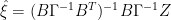
Brown’s inconsistency R (denoted here sometimes by Rb) is defined as follows (with the hat denoting the GLS fit rather than the maximum likelihood fit) and $\hat{B}$ being the same thing as the B obtained above (the hat being assumed in this frequently used object).

At 1987 page 56, Brown and Sundberg give the results for three cases, which you may also calculate directly as follows (which I present as evidence that my implementation of the Brown inconsistency diagnostic has been done correctly, prior to describing its calculation. Brown considers the significance of this statistic relative to a chi-squared distribution (df=1 here) and the implied chi-squared values are also shown.

Rb(Z=c(1.68,38.64)-Basics$ybar) #case a brown[18,]
# 0.825 versus reported 0.83
Rb( Z=c(1.86,35.7) -Basics$ybar) #case b
# 4.46 versus reported 4.46 #said to be significant at 5% level
Rb (Z=c(1.94,34.09)-Basics$ybar);#case (c)
# 13.14 versus reported 13.14
#said to be significant at 0.1% level based on chisq df=1
qchisq(c(.95,.99,.999), df=1)
# 3.841459 6.634897 10.827566

The calculation of the inconsistency R can be seen in the functions. While there seemed to be some other candidate denominators for the calculation of $\hat{\Gamma}$ , the following seemed to work (note that the definition of $\hat{\xi}$ is structurally identical to MBH, except that MBH replaces the GLS estimator $\hat{\Gamma}^{-1}$ with arbitrary weights and Wahl and Ammann 2007 with the identity matrix I. Using l here to denote the number of rows in the individual estimate (typically 1 for each year in proxy situations, but the methods can be adapted to an entire verification period):

$\hat{\Gamma}=S/(n-p-q)$ from 1987 2.11
$\hat{\xi}=(B\Gamma^{-1}B^T)^{-1}B\Gamma^{-1}Z$
$R=||Z-\hat{\xi}B||_{\hat{\Gamma}^{-1}}^2$ which is merely notation for

$R= (Z-\hat{\xi}B) \hat{\Gamma}^{-1} (Z-\hat{\xi}B)^T$

I’m not clear why the GLS estimator $\hat{\xi}$ is used here instead of the maximum likelihood estimator $\tilde{\xi}$ (denoted by Brown with a double-hat (which will be described below). The double-hat doesn’t render here and so the tilde is used.

Confidence Intervals and the Inconsistency Diagnostic
Brown and Sundberg 1987 show that the likelihood-based confidence interval in multivariate calibration expands dramatically as Rb increases.

First is their Figure 1 and then is my emulation, which visually matches and, as discussed below, there are benchmark matches as well. In the examples shown here, the GLS estimate $\hat{\xi}$ is arbitrarily set at 1 and the profile maximum likelihood is then calculated. As observed by Brown and Sundberg, the maximum likelihood estimate $\tilde{\xi}$ (the minimum here) coincides with the GLS estimate only when Rb=0. As Rb increases, it goes increasingly far away from $\hat{\xi}$ . This is something that needs to be borne in mind by people who worry about the standard deviation of reconstruction time series – it would be noticeably higher in a maximum likelihood reconstruction (I’ve done some preliminary analyses).

For benchmarking purposes, Brown and Sundberg report the confidence intervals for each of these four figures, which are matched up to rounding in my emulation (thumbnails shown below):

The widening of the confidence intervals with increasing inconsistency diagnostic R(b) is really quite dramatic. It doubles when R=4 and becomes almost infinite when R=7; when R=20, one has a very perverse situation (which has been noted for a long time in univariate calibration e.g. Fieller 1954 and many others.

-0.98	4.1
-0.85	71.58
-1.02	8.51
2.6	-8.4

Having established that I’ve replicated this particular Brown and Sundberg 1987 procedure, what is it operationally? This calculation originates with the profle likelihood equation set out in 1987 equation 2.14:

After some manipulations, Brown and Sundberg report that this can be re-written as proportional to (and thus the same maximum likelihood estimator):

The element m in this equation is a function of the degrees of freedom: m=(n-p-q) (n+1)/n. The above form (1987 equation 3.6) with simplifications available for the case of one-dimensional X is implemented in R as:

f=function(mu,R) (R+ (mu-muhat)^2)/(1+g*mu^2) ##see ff eq 3.10
#muhat and g are pre-set

Because the maximum likelihood functions have a well-defined shape, the location of the minimum is easily obtained numerically in R using the flexible and efficient optimize function (Brown and Sundberg also show an analytic calculation.) Here I show the implementation within my wrapper function for R=4.

test=optimize(f,c(0,20),tol=0.001,R=4);unlist(test)
#minimum objective
# 1.531 3.469

The maximum likelihood estimate is the first item (called “minimum” in R, but this is the x-location of the minimum, while the “objective” is the y-value of the minimum. The second argument in the function is the interval over which the optimization is specified. Here I know what’s needed to cover the answers and have specified it. In other cases, I’ve experimented with 3 times the range of the x-values in the calibration period and that seems to work. Note that the maximum likelihood value has already changed quite a bit from the GLS (Mannian) value of 1 and this changes quite a bit as Rb gets higher (the proxies get more inconsistent).

The next operation in the calculation of likelihood-based confidence intervals is the calculation of the level of the dashed line in the above figures, which represents the 95% coverage level (and thus a likelihood based confidence interval.) This is defined in 1987 equation 4.3 as follows, with ${ \hat{\hat{\mu}}$ being the maximum likelihood estimator:

In my R script, this has been implemented in log form through the function shown below (where kgamma is the 95 percentile chi-squared value defined by kgamma=qchisq(.95, df=p):

cstar=function(R) (m+f(muhat,R)) * exp(kgamma/(n+1)) -m

The confidence intervals could easily be calculated numerically as the intersect of this vertical level with the likelihood function. Brown and Sundberg 1987 derive an analytic formula shown below (1987 equation 4.4) based on solutions to a quadratic equation. This formula is helpful because it shows how the confidence interval becomes imaginary, an approach which is used in my R-function cstar.brown.

Brown and Sundberg Figure 2
There is one other benchmarking calculation: Brown and Sundberg Fig 2, shown below together with my emulation, showing the profile likelihood for the three cases for which the Inconsistency R was calculated above. Here is the original figure followed by my emulation:

Brown and Sundberg Fig 2 and emulation.

Visually they appear identical. Brown and Sundberg give information on the confidence intervals shown by the dashed lines and my calculation matches these exactly, confirming that this implementation is also accurate. The curves plotted above are the profile likelihoods for the three different proxy combinations (leading in each case to the maximum likelihood estimator). As indicated in the original legend, this is based on 1987 equation 2.14 which is

This was a bit fiddly to figure out, since Brown and Sundberg elsewhere say that, in the case of just one reading of the proxies (the case in examples that interest us), the S matrix in the denominator is the calibration S matrix without pooling, although the language here certainly indicates pooling. For calculation purposes, the one is as easy as the other. I got the results to match in the case where l= 1 without pooling so I presume that this is the proper interpretation. (see the function profile.lik in the scripts for this step.)

I then determined the maximum numerically by the optimize function. The dashed line showing the 95% confidence interval is set at kgamma/2 below the maximum (kgamma defined from the chi-squared distribution above.) I then solved for the two end-points of the confidence interval calculation numerically by equating the vertical level to the likelihood function. The benchmarking is exact.

I’ve posted up a note reconciling three different forms of expressing profile likelihoods in Brown and Sundberg 1987 here

At a later date, I’ll show what happens when you start applying these methods to proxy studies. It’s pretty interesting. You can see the direction that this is going to go: Inconsistency R statistics on a year-by-year can be calculated for each of the proxy networks regardless of whether they are CPS, Mannian or correlation-weighted. This approach also leads to “honest” confidence intervals (to borrow a phrase from an econometrics article) as opposed to the irresponsible use of calibration residuals in Mannian/Ammannian calculations, something that I think may lead to a far more definitive treatment of these networks. Finally I think that there is a way of getting at the RE bilge because the methods can be used for verification sets where l exceeds 1. So I think that these simple tools may be pretty useful.

Brown, P. J. 1982. Multivariate calibration. Journal of the Royal Statistical Society, Series B 44: 287-321.
Brown, P. J., and R. Sundberg. 1987. Confidence and conflict in multivariate calibration. J. Roy. Statist. Soc. Ser. B 49: 46-57.
—. 1989. Prediction diagnostics and updating in multivariate calibration. Biometrika 76, no. 2: 349-361. url

This entry was written by Stephen McIntyre, posted on Jul 30, 2008 at 7:24 PM, filed under Statistics and tagged brown, calibration, multivariate, sundberg. Bookmark the permalink. Follow any comments here with the RSS feed for this post. Both comments and trackbacks are currently closed.

19 Comments

Steve McIntyre

Posted Jul 30, 2008 at 8:03 PM | Permalink

Here is the script for this article:

#BROWN AND SUNDBERG 1987 exampe

####FUNCTIONS
url=”http://www.climateaudit.org”
source(file.path(url,”scripts/brown/functions.brown.txt”))

##Paint Data
Paint=read.table(file.path(url,”data/brown/Paint.brown.dat”),sep=”\t”,header=TRUE) #this table has been organized in nrown/collation.paint.1982.txt
brown=Paint
calibration=(1:nrow(brown))[Paint$ver==”cal”]; n=length(calibration);
verification=(1:nrow(brown))[Paint$ver==”ver”]; l=length(verification);
Y=as.matrix(brown[calibration,c(“Y1″,”Y4″)])
X=as.matrix(brown[calibration,”viscosity”])
Xver=as.matrix(brown[verification,”viscosity”])
Z0=as.matrix(brown[verification,c(“Y1″,”Y4″)]);#see 1987 page 56
Z0

##EXECUTE WRAPPER OPERATIONS
Basics=brown.basics(X,Y,Z0,Xver)
Profile=brown.profile(Z0,Basics,Xver)

###BENCHMARKING
options(digits=4)
Basics$ybar #matches 1987 p 56
# Y1 Y4
# 1.747778 37.936296

Basics$B #mathces 1987 p 56
# Y1 Y4
#[1,] -0.128 -1.69

Basics$Sinv
# Y1 Y4
#Y1 6.86285 0.03052
#Y4 0.03052 0.02299

#inconsistency function
Rb(Z=c(1.68,38.64)-Basics$ybar) #case a brown[18,]
# 0.825 versus reported 0.83
Rb( Z=c(1.86,35.7) -Basics$ybar) #case b
# 4.46 versus reported 4.46 #said to be significant at 5% level
Rb (Z=c(1.94,34.09)-Basics$ybar);#case (c)
# 13.14 versus reported 13.14
#said to be significant at 0.1% level based on chisq df=1
qchisq(c(.95,.99,.999), df=1)
# 3.841459 6.634897 10.827566

###############
### FIGURE 1 #Brown 1987 page 53
#reported data in article
fig1.int=t( array(c(-0.98,4.10,-1.02,8.51,-.85,71.58, 2.6,-8.4),dim=c(2,4)))
fig1.int=fig1.int[c(1,3,2,4),];fig1.int
#maketable(fig1.int)
#collect information for profile likelihood calculations
n=Basics$n;
p=1; g0=0.1;g=0.1;muhat=1
p=1; q=4;n=50 ## see Brown 1987 page 54 bottom para
n0=n-p-q;n0 #45
m=n0* ((n+1)/n) ;m# eq 3.3 #45.9
kgamma=qchisq(.95, df=p);kgamma#3.841459
R0=c(0,7,4,20)
f=function(mu,R) (R+ (mu-muhat)^2)/(1+g*mu^2) ##post 3.10
#muhat and g are set arbitrarily above (but not in application)

#calculate confidence intervals
ci=array(NA,dim=c(4,2))
cstar.fig1=rep(NA,4)
for (i in 1:4){
R=R0[i]
test=optimize(f,c(0,20),tol=0.001,R);unlist(test)
mu.double=test$minimum;mu.double #0.999984
cstar.fig1[i]= cstar(R,mu.double); # 3.590852
mu0=-1/g0/mu.double;mu0 # -10.00016
ci[i,]=cstar.brown(R,cstar0=cstar.fig1[i]);#-1.007928 4.162480 #reoprted -0.98 4.10 p54
}

#illustrate one of the steps in above iteration
test=optimize(f,c(0,20),tol=0.001,R=4);unlist(test)
#minimum objective
#1.531 3.469
cstar(R=4,test$minimum);#7.331

cstar.fig1 #these are the confidence lines
#[1] 3.591 9.719 7.331 13.463

ci #these match re[prted values
# [,1] [,2]
#[1,] -0.9847 4.105
#[2,] -0.8493 71.985
#[3,] -1.0253 8.519
#[4,] 2.5990 -8.375

##CA PANEL FIGURE 1
nf=layout(array(1:4,dim=c(2,2)))
xlim0=c(-15,25); xx= seq(-15,25,.5);ylim0=c(-1,26)
for (i in 1:4 ){
par(mar=c(2,2,2,2))
plot(xx,f(xx,R0[i]),type=”l”,xlim=xlim0,ylim=ylim0);abline(h=0,lty=3);abline(v=0,lty=3)
if(ci[i,2]>ci[i,1]) {lines(xy.coords(ci[i,],rep(cstar.fig1[i] ,2)),lty=2)} else {
lines(xy.coords(c(ci[i,1],1000),rep(cstar.fig1[i] ,2)),lty=2)
lines(xy.coords(c(-1000,ci[i,2]),rep(cstar.fig1[i] ,2)),lty=2) }
points(xy.coords(ci[i,],rep(cstar.fig1[i] ,2)))
text(-15,25,paste(“R=”,R0[i]),font=2,pos=4)
if(i ==3) mtext (at= -20, “Brown 1987 Figure 1″, line=0.7, font=2)
}

##########################
########################
#this is a 3-panel figure illustrating likelihood for 3 different Z-combinations – see page 56

xx=seq(-2.5,2.5,.1);xlim0=c(-2.5,2.5);ylim0=c(-10,0)
gx=function(xx,Z){N=length(xx);gx=rep(NA,N);for (j in 1:N) gx[j]=profile.lik(xx[j],Z);gx}
bx=function(xx,Z){N=length(xx);bx=rep(NA,N);for (j in 1:N) bx[j]=brown.lik(xx[j],Z);bx}
#these functions just calculate values for the plot-vector. This can probably be done in one vector.

fig2.int=t(array(c(-.76,1.12,-1.08,.97,-1.34,1.16),dim=c(2,3)))
#this is the reported data.
Zb=t(array(c(1.68,38.64,1.86,35.70,1.94,34.09),dim=c(2,3)) )
Zcentered=scale(Zb,center=Basics$ybar,scale=FALSE)
#the same examples as in the Rb function
c0=rep(NA,3)
xlim0=c(-2,2);xrange=3*range(Profile$stat$xhat)
fig2.stat=array(NA,dim=c(3,2))

#PLOT FIGURE 2
nf=layout(array(1:3,dim=c(1,3)),widths=c(1.1,1,1))
for(i in 1:3) {
par(mar=c(3,3,2,1))
Z=Zcentered[i,]
test=optimize(profile.lik,xrange,tol=0.001,Z,maximum=TRUE);unlist(test)
c0[i]=test$objective-kgamma/2;c0[i] # -2.362005
h=function(x) (profile.lik(x,Z)-c0[i])^2
testl=unlist(optimize(h,c(xrange[1],0),tol=0.001));testl
testu=unlist(optimize(h,c(0,xrange[2]),tol=0.001));testl
fig2.stat[i,]=c( testl[1],testu[1])

plot(xx,gx(xx,Z),type=”l”,ylim=ylim0,xlim=xlim0,ylab=””,xaxs=”i”)
abline(h=c0[i],lty=2)
if(i==1) mtext(side=2,line=2,”Log Likelihood (2.14)”,cex=.8,font=2)
if(i==2) title(“Brown and Sundberg 1987 Fig 2”)
text(-2,0,font=2,pos=4,paste(“Z=”,Zb[1],Zb[2],sep=” “))
}

#show that calculated intervals match reported intervals
round(data.frame(fig2.int,fig2.stat),2)
# X1 X2 X1.1 X2.1
#1 -0.76 1.12 -0.75 1.12
#2 -1.08 0.97 -1.07 0.97
#3 -1.34 1.16 -1.34 1.16
Pat Frank

Posted Jul 30, 2008 at 8:44 PM | Permalink

Steve, I have nothing but profound admiration for your work and for the high level of scientific and statistical rigor you’ve brought to the field of proxy climatology. The project you describe here is also nothing short of admirable and, with respect to the current crop of academic practitioners, shamefully overdue.

That said (and you knew this was coming) I hate to be a fly in that precious ointment, but the entire problem with tree ring paleothermometry is this: “The problem is that the error bars have no statistical meaning and provide a faux confidence in the results.”

The problem is that in the absence of a physical theory, even completely sound statistical confidence limits have no physical meaning and provide no scientific import to the results.

There is as yet no physical theory from which one can derive a temperature from a tree ring. The PCA and renormalization method (and that’s all it really is) does nothing to turn ring widths into physically meaningful temperatures. The garbage confidence limits currently plaguing the field of tree ring paleothermometry are statistical garbage attached to scientific garbage.

Rectifying the statistics won’t rectify the science. The major problem with tree-ring paleothermometry is that it presently is false science.

An exception can be made, in principle, for temperatures derived from O-18 fractionation, which has a fine physical theory, but which has yet to be applied successfully to tree rings.

If this post is OT with respect to your desired conversation, please do go ahead and move it to unthreaded.

Steve: Let’s have this comment for the record (and it’s one that I agree with). But I really don’t want people piling on with more griping about tree rings. We know all that. What I want to do with this material is a little different: demonstrate just how wide are properly calculated CIs with these data sets, even if there was a physical connection, by which one bristlecone could act as a thermometer for Asia, another a few feet away for Africa and another over the hill for Peru.
Leonard Herchen

Posted Jul 30, 2008 at 8:53 PM | Permalink

Steve:
I, or better put, people smarter than me who I work with, are using a program called discipulus from http://www.rmltech.com. We look at commodity price time series and related data. It doesn’t come in a pretty package but works for us. I suspect it may be useful in this problem. It does what it calls genetic programming. It is fairly simple and fast. Have a quick look at their website to see if it may help you.
Your commitment to valid science is inspiring.
DeWitt Payne

Posted Jul 30, 2008 at 9:39 PM | Permalink

The company I worked for spent a lot of time and money a while back trying to get NIR multivariate calibration using filter instruments to work as in line and off line process analyzers. It was largely a failure. OTOH, the biodiesel industry is currently using Fourier Transform-IR spectrophotometers for process analysis (free and total glycerin, cetane number, etc.) and it seems to work quite well. I don’t think they’re using classical chemometric multivariate analysis though. I don’t really know because the system I am familiar with used an off site proprietary database to calculate results from spectra transmitted over the internet.
Ross McKitrick

Posted Jul 31, 2008 at 12:38 AM | Permalink

Great work mapping Brown et al into R code and concrete computational steps Steve!

CA Readers: It might be helpful, by way of background, to emphasize that the underlying statistical problem involves regressing [proxy Y] on [temp X], then using Y to forecast X out of sample. Early on in the calibration lit Krutchkoff (1967) asked why not regress X on Y. This can be rationalized if the problem is re-cast as a Bayesian inference, but the literature flowing from Brown (1982) rejects this if (i) there is a clear causality from X to Y, rendering the ‘X-on-Y’ regression inconsistent, and (ii) you want to forecast outside the sample range.

Faced with the problem of estimating X-hat, Brown tackled the problem back-to-front. Deriving a point estimate and standard error, then proposing X-hat +/- 2SD, doesn’t work because the underlying theory doesn’t establish that 2SD encompasses 95% of the probable values. Instead Brown derived a 95% confidence interval, then collapsed it to a point to get the point estimator.

Some further refinements to this method dealt with problems in his proposed 95% CI. One of them is that the CI in Brown (82) is not invariant to simple translation of the data (Steve — does that apply to B&S 87? it didn’t come up AFAIK until Oman’s 1988 paper). Another is that under some circ’s the CI can shrink the greater is the inconsistency measure, indicating CI shrinkage is not a good indicator of model quality.

In the B&S 1987 paper discussed above, they dealt with the estimation problem in a clever way, by deriving MLE parameters assuming the unknown point estimate is known, as well as deriving an expression for the MLE with the point estimator unknown but written so that it must be max’d when the estimator = 1. Then they form the ratio of these two and the result at the ML value is called the “profile MLE estimator”.

Where all this is eventually heading is that Steve will be able to generate confidence intervals for paleoclimate recon’s that actually have statistical theory behind them, not just stupid ad hoc handwaving.
There is one particularly juicy little result lurking out there by Gleser and Hwang in 1987 which hopefully will be the basis of a future post, and possibly some interesting graphs.
UC

Posted Jul 31, 2008 at 12:50 AM | Permalink

This is very helpful! I get R values for Brown87 cases

a) 0.8247

b) 4.4565

c) 13.1400.

GLS estimates

a) 0.1718

b) -0.0445

c) -0.0726

..but my classical intervals are slightly off,

a) -1.0304 … 1.4048
b) -0.8335 … 0.7364
c) empty

Probably due to inefficient minimum location search algorithm I use.

I still need to update these CIs

http://signals.auditblogs.com/2007/07/09/multivariate-calibration-ii/

with newer code, but I guess the direction will be the same; very difficult to claim unprecedented 20th century with this data..
John A

Posted Jul 31, 2008 at 4:03 AM | Permalink

Ross:

Where all this is eventually heading is that Steve will be able to generate confidence intervals for paleoclimate recon’s that actually have statistical theory behind them, not just stupid ad hoc handwaving.

There are several points I’d like to make:

1. Before calibration can even begin, the physical causality of tree ring width/maximum densities and ambient temperature (never mind the magic of detecting the global temperature field from Colorado) must be established, not simply assumed to be true. There was a recent report which shows that tree leaves stay at nearly a constant temperature regardless of the ambient temperature, trashing one of the most cherished assumptions of dendroclimatologists.

2. I missed this in the post above, but how are confidence limits dealt with in datasets with high autocorrelation?

3. And what about non-linear responses?

4. Although Steve will probably dislike me for saying it, it would be better all round for Steve to put some of his most significant posts into a letter or article in a quality professional journal (and I don’t mean Science or Nature). For example, these posts on tree ring networks and Toeplitz matrices deserve submission to a good statistical journal rather than just lingering as blog posts. Such submissions might actually stimulate the statistical community to provide more feedback into the questions above and how to go about solving them.

My 2c
MrPete

Posted Jul 31, 2008 at 5:53 AM | Permalink

John A (and lurking Pat Frank 😉 ), I believe it’s reasonable to begin within an assumption of physical causality, and see what kind of CI’s you get with rigorous math/stats. If the CI range is floor to ceiling, then it doesn’t matter whether physical causality can be proven.

Just as with Geoff’s example, proxies aren’t going to give any better results than the real world.

I’m reminded of this every time I look at our weather forecast. They give some detailed figures for the next 24 hour period, but then the forecast quickly devolves to a standard hi/lo range based on historical averages. Their predictors just aren’t any better than that.

So too here. If I’m not mistaken, Steve is developing the math/stats for determining best case confidence intervals. Those who have been claiming more “robust” confidence will need to step back and prove their assertions. You can’t “move on” when your foot is caught in a trap.
John A

Posted Jul 31, 2008 at 6:31 AM | Permalink

Then putting the case here can only be the first step in getting them into the literature. Then watch the Team try to “Move On”

But the problem is that unless physical causality has been established, spurious correlation between unrelated time series is an ever present concern
Steve McIntyre

Posted Jul 31, 2008 at 8:07 AM | Permalink

Please, I don’t want people piling on with comments about cherrypicking or causality. It’s not like I’m unaware of these issues. Those are valid lines of argument, but please bite your tongues.

And yes, this is the sort of thing that I’m inclined to work up for publication in a technical publication. It’s something that I’ve been working at on and off for a long time and only recently got a secure foothold on Brown and Sundberg. The approach that this leads to is clearly fresh and distinctive, and will lead to new perspectives without being argumentative.
Steve McIntyre

Posted Jul 31, 2008 at 1:15 PM | Permalink

UC has an interesting post and here last summer on this matter that I’ve now linked in the post (and should have linked earlier).

The approach taken here differs from the approach taken in UC’s post. UC uses the methods described in Brown 1982 for CIs, while I’ve used the later method in Brown and Sundberg 1987, which looks like an improvement over the earlier method. I’m pretty sure that we can tie things back and forth and we’re definitely making progress!
William Newman

Posted Jul 31, 2008 at 4:36 PM | Permalink

John A. writes “1. Before calibration can even begin, the physical causality of tree ring width/maximum densities and ambient temperature (never mind the magic of detecting the global temperature field from Colorado) must be established, not simply assumed to be true.”

I don’t think that should be an absolute rule. It’s probably a useful rule of thumb when small hand-collected datasets meet the data mining capability of modern CPUs. But think what happens when our modern CPUs meet enormous data sets from modern automated instruments. If someone discovers a very strong correlation in terabytes of genomic data or astronomical observations, it’s fairly likely to be something real even if we don’t yet have the foggiest idea why.

(It should be possible to quantify the risk of overfitting, instead of just making a yes/no binary rule of thumb. I’m vaguely aware of two ways to do so. However, I’ve never used either. Thus, to reduce my risk of saying something unusually dumb, I’ll leave constructive suggestions to others.)
bender

Posted Aug 1, 2008 at 12:42 AM | Permalink

What is it compels people to ruin technical threads like this? STOP PISSING ON THE LAB NOTEBOOK, PEOPLE.

Steve: I made the following request above:

Please, I don’t want people piling on with comments about cherrypicking or causality. It’s not like I’m unaware of these issues. Those are valid lines of argument, but please bite your tongues.

I’m going to be pretty strict in what remains in this thread. If you want to post something other than technical or if you want to debate tree rings, then assume that the comment is going to be transient in the record or going to Unthreaded. I’ve already done this with some posts which had transient interest; I’m just going to try to keep a fairly coherent comment thread, that’s all.
UC

Posted Aug 1, 2008 at 3:32 AM | Permalink

John A (13)

1. Before calibration can even begin, the physical causality of tree
ring width/maximum densities and ambient temperature (never mind the
magic of detecting the global temperature field from Colorado) must
be established, not simply assumed to be true. There was a recent
report which shows that tree leaves stay at nearly a constant
temperature regardless of the ambient temperature, trashing one of
the most cherished assumptions of dendroclimatologists.

Sure, one should not attempt calibration when one is not confident that $\beta \neq 0$ ( Brown82 ) . And our ideas on causation must come from outside statistics (any stat book).

2. I missed this in the post above, but how are confidence limits dealt with in datasets with high autocorrelation?

Brown assumes that errors are uncorrelated over time, Brown 87 Eq 2, i is annual time index in tree-ring case. Mann has some tools for redness estimation and correction ( http://www.climateaudit.org/?p=1810 )
Steve McIntyre

Posted Aug 1, 2008 at 9:36 AM | Permalink

I’ve posted up a note reconciling three different forms of expressing profile likelihoods in Brown and Sundberg 1987 here
John Baltutis

Posted Aug 1, 2008 at 4:10 PM | Permalink

Re: #15:

The equations don’t display in your linked article. Both in my browser and when I download it.
John A

Posted Aug 1, 2008 at 8:52 PM | Permalink

I concur with John Baltutis, the equations are missing.
Willis Eschenbach

Posted Aug 2, 2008 at 1:47 AM | Permalink

I’m not sure I completely understand the inconsistency statistic. Suppose someone used say the 8 various temperature records used by Koutsoyiannis, as proxies for this type of analysis. What exactly would a high inconsistency statistic of these records mean in some physical sense? What would a low statistic mean?

w.

Steve: More to come.
UC

Posted Aug 4, 2008 at 7:03 AM | Permalink

Willis #18,

Interesting question. If one calibrates 8 independent proxy series to their mean, S-matrix ( see the next thread) will be singular, but not zero matrix. The calibration algorithm sees correlated noise between proxies, even though there was no noise at all. Might cause some trouble.

But if you have the mean of the temperatures available, you also have the individual local temperature records. And calibration locally would make much more sense, as one looses information in the averaging process. If it is assumed that proxies directly respond to global average (*) , then we can use R safely.

(*) sun sensor, CO2 sensor, PC1, for example 😉