Climate Audit

When Wahl and Ammann’s script first came out, I was able to immediately reconcile our results to theirs – see here. As Wegman later said:

when using the same proxies as and the same methodology as MM, Wahl and Ammann essentially reproduce the MM curves. Thus, far from disproving the MM work, they reinforce the MM work.

You’d never know this from Team and IPCC accounts of the matter, but this is actually the case. The most recent Wahl and Ammann fiasco with their RE benchmarks is merely one more example.

While they archived their code (excellent), it wasn’t set up to be turnkey, nor is their most recent code. My own code at the time wasn’t turnkey either, since my original concept in archiving code was really to provide documentation. However having started down that road, it’s not much extra time or trouble to make things turnkey and, aside from the convenience to readers, there are considerable advantages for one’s own personal documentation in buttoning up code so that it’s turn key. When I picked up this file again in connection with the recently archived Ammann SI, I re-visited my script implementing Wahl and Ammann’s code. I modified it slightly to make it turnkey.

I also modified it slightly so that I could readily prove that our results reconciled exactly to theirs, also with turnkey scripts, as I reported in May 2005. This reconciliation is demonstrated below on a line by line basis, which also serves to illuminate the structure of the calculations in a useful way.

I’ve placed the following script online here.

First, the following text calls on my implementation of Wahl and Ammann code in one line. You can examine the code if you look.

source(“http://data.climateaudit.org/scripts/wahl/mann_masterfile.windows.txt”)

It takes a little while to work and when finished, will note on the console that it has “Read 1 item. Read 2 items.,,,, etc.” It creates directories in your d: drive. If you don’t have a d: drive, manually edit the references in the script from d: to c:. This results in an R-list wahlfit with 11 items, one for each of the 11 MBH steps from 1400 to 1820 (1400 first).

The script prints out a few entries so that you can confirm that you’ve got the right object.

W=wahlfit[[1]];
W[[2]]$TmatD[1:4]
#1] 154.02858 75.17558 63.15213 61.86446
attributes(W[[2]])
#$names
#[1] “TmatU” “TmatV” “TmatD” “TmatD.truncated”
#[5] “ctrs.TmatU.ret.anom.cal” “stds.TmatU.ret.anom.cal” “TmatU.ret.anom.cal” “TmatV.truncated”

Next the script demonstrates the reconciliation of my linear algebra with Wahl and Ammann’s verbose and obscure code (which improves on the even more verbose and obscure original code. First, I collect some of the relevant targets from within Wahl and Ammann code (made possible by collecting the objects into an R-list). The AD1400 step is in wahlfit[[1]] so we start our reconciliation there, first labelling that step, then collecting the proxy network, the reconstruction and the temperature PC1, giving each of them short names for further steps.

W=wahlfit[[1]];#names(W)
proxy=ts( wahlfit$”1400″[[1]]$Ymat.anomaly,start=1400);dim(proxy)
# 581 22
recon=ts(c(wahlfit$”1400″[[3]]$Tmat.anomaly.precal.fitted.NH.mean.corrected,wahlfit$”1400″[[3]]$Tmat.anomaly.cal.fitted.NH.mean.corrected),start=1400);length(recon)
#583 #this is WA version
pc=wahlfit$”1400″[[2]]$TmatU[1:79,1:16] ;pc[1:5,1] #WA pc
#-0.04026887 -0.09598517 -0.17558648 -0.08449567 -0.03783115

Next we do a little linear algebra to collect the weights of each reconstructed temperature PC in the final NH temperature reconstruction. (I showed a couple of years ago that a calculation involving hundreds of thousands of calculations every time you picked up the file, could be done once as the MBH/WS recon is a linear combination of the reconstructed PCs with weights that do not vary (other than whether they are included or excluded. The following implements this linear algebra in one line:

weights.nh=diag(W[[2]]$TmatD[1:16]) %*% t(W[[2]]$TmatV[nhtemp,1:16])%*% diag(W[[1]]$stds.Tmat.anomaly[nhtemp])%*%as.matrix(W[[1]]$grid.cell.stds[nhtemp])/sum(W[[1]]$cos.lat.instrumental[nhtemp])
c(weights.nh)[1:5]
# [1] 1.81831789 -0.48908006 0.08932557 0.53319471 0.08284691

The reconstruction itself also has very simple linear algebra – underneath all the inflated talk of maximizations and minimizations. This was a point that we emphasized as early as MM03. Wahl and Ammann have applied many of the same techniques, though, in my opinion, with some deterioration in insight, as they don’t seem to think naturally in algebraic terms. This linear algebra was posted up at the blog several years ago. In baby steps, here is the reconstruction calculation (

First, we collect the proxies (Y) and the temperature PCs (X) and scale them in the calibration period (1902-80).

ipc=1; N=nrow(proxy)
m0=apply(proxy[(N-78):N,],2,mean);sd0=apply(proxy[(N-78):N,],2,sd)
Y=scale(proxy,center=m0,scale=sd0)
X=as.matrix(pc[1:79,1:ipc]) # 0.02310907
sd.obs=apply(X,2,sd)
index=(N-78):N #the calibration period

Next we use equal weights (following WA; Mann used arbitrary weights – I have no idea how he assigned these weights.) Mannian methods result in the weights being squared (which is unexpected and unreported). It doesn’t “matter” with equal weights which might explain why WA failed to follow MBH on this step in their benchmarking. It was not easy to figure out that Mannian code ended up squaring the weights.

weightsprx=rep(1,ncol(Y))
P=diag(weightsprx)^2

Next we calculate the vector of correlations of each proxy to the PC1. I implemented this way in the 1-D case to show the commonality of this approach to correlation-weighted methods, believed by their proponents to be different than MBH

rho=t(as.matrix(cor(pc[1:79,1:ipc],Y[(N-78):N,]))); #16 19

Mann then has a seemingly ad hoc re-scaling of the temperature PCs to the observed PCs. This has been a troublesome feature for people trying to replicate his results because it’s not mentioned anywhere in th original text; it seems to have been a stumbliing for Wahl and Ammann as well, because although they claimed that their implementation was free-standing, their code acknowledges a pers. comm. from Mann on this point. In our early code, this step was done in a purely empirical way, as Wahl and Ammann do as well. However, it turned out that this operation can also be expressed simply in linear algebra, which I’ve done here. This took me an undue amount of work a while ago to figure out and, aside from simplifying code, it is useful in laying bare the structure:

sd.est = sqrt(diag( t(rho)%*%P %*% t(Y[index,])%*% Y[index,] %*% P %*% rho) ) /sqrt(78) ;
sd.adj=as.matrix( sd.obs[1:ipc]/sd.est[1:ipc])

Now the reconstructed temperature PC1 can be calculated in one line of linear algebra (I use the notation Uhat for the reconstructed PC1 since it is an estimate of the target temperature PC U):

Uhat = Y %*% P %*% rho %*% diag(sd.adj)

From this reconstructed PC1 and the vector of weights calculated previous, we can calculate the NH reconstruction for this step in one line, labelled tau below.

tau= ts(Uhat %*% weights.nh[1:ipc,],start=tsp(proxy)[1])

In case it’s useful, I also calculate the weights (beta) of the individual proxies in the reconstruction, which can also be done in one line:

beta= P %*% rho %*% diag(sd.adj) %*% weights.nh[1:ipc,]

Doesn’t look much like the hundreds of lines of Fortran code. (UC’s Matlab implementation is in the same spirit though it has nuances of difference.)

Could something done so simply actually reconcile to Wahl and Ammann. Well, we collected their reconstruction for the AD1400 step above, so let’s calculate the maximum difference between the two series:

max(tau-recon) # 1.165734e-15

Bingo. I’ve collected the above operations into a function which requires three parameters – the proxy, the weights and the number of temperature PCs. This matches.

test=mannian(proxy,weightsprx=rep(1,ncol(proxy)),ipc=1)
max(test$series-recon) # 1.165734e-15

You can now plot the result:

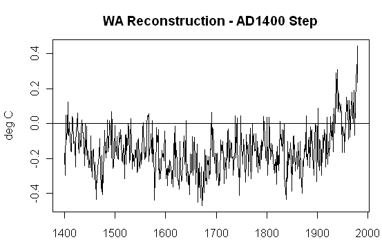
par(mar=c(3,4,3,1))
plot(1400:1980,test$series,type=”l”,main=”WA Reconstruction – AD1400 Step”,xlab=””,ylab=”deg C”)
abline(h=0)

This should give you the following.

Sparse
The following shows how easily the “sparse” calculation can be implemented if one thinks about it logically. Mann defines a subset of 212 gridcells for verification (his “sparse” ) set; these locations are not mentioned anywhere. I blew up the Nature diagram to try to figure it out; Wahl and Ammann have an index list of NH sparse gridcells, which I’ve collected as sparse.index below. As with the NH reconstruction, the sparse reconstruction is a linear combination of reconstructed PCs and the weights can be calculated in one go in an identical manner as with the NH weights as follows:

weights.sparse=diag(W[[2]]$TmatD[1:16]) %*% t(W[[2]]$TmatV[sparse.index,1:16])%*% diag(W[[1]]$stds.Tmat.anomaly[sparse.index])%*%as.matrix(W[[1]]$grid.cell.stds[sparse.index])/sum(W[[1]]$cos.lat.instrumental[sparse.index])
c(weights.sparse)[1:5]
# 1.6215193 -1.1292956 0.5358274 0.5652639 0.3264116

The estimate for the sparse region can then be calculated in one line as well:

sparse_est= ts(Uhat %*% weights.sparse[1:ipc,],start=tsp(proxy)[1])

Note that in this case, all that happens is that one weight differs a little bit, as only the first weight is used. The constant 1.62152 is used for the sparse estimate, as compared to 1.81831789 for the NH calculation, which attenuates this a little. I’ll show that this also reconciles exactly, but first something odd has to be watched out for. In constructing their calibration-verification combination, Wahl and Ammann don’t calculate calibration and verification statistics consistently on the same data set. They splice the estimate for the “dense” subset in the calibration period with the estimate for the “sparse” subset in the calibration period. If these two things are spliced, you get a perfect match as shown below:
range(W[[3]]$estimator- c(sparse_est[(1854:1901)-1399],recon[(1902:1980)-1399]) )
#] -2.775558e-16 1.665335e-16

The function that I’ve used for the past few years (not as pretty as I’d do it now, but serviceable), gets identical calibration RE and verification RE scores, apples and apples:

verification.stats(observed=W[[3]]$observed,estimator=W[[3]]$estimator,calibration=c(1902,1980),verification=c(1854,1901))
# RE.cal RE.ver R2.cal R2.ver CE
#1 0.3948435 0.4811857 0.4135687 0.01819374 -0.2153968
W[[3]]$beta
#1] 0.0599089 0.3948435 0.4811857

Now here’s something for connoisseurs of Texas sharpshooting. What would happen if we did both calibration and verification on the same data set. On an earlier occasion, I extracted the target sparse data set. Instead of splicing two different series, let’s look at calibration and verification on the same time series. This time the calibration RE is only 0.177 (!), while the verification RE still rounds to 0.48 (I guess there are probably rounding differences in this somewhere accounting for the slight difference in verification RE values).

download.file(“http://data.climateaudit.org/data/mbh98/sparse.tab”,”temp.dat”,mode=”wb”);load(“temp.dat”)
#load(“d:/climate/data/mann/sparse.tab”)
verification.stats(observed=sparse[,1],estimator=sparse_est,calibration=c(1902,1980),verification=c(1854,1901))
# RE.cal RE.ver R2.cal R2.ver CE
# 0.1777026 0.4782771 0.1877987 0.01823145 -0.2229820

The ratio of calibration RE to verification RE, apples and apples, is only 0.37, well below even the redneck ratio of 0.75.

The function is as follows:

mannian=function(proxy,weightsprx=rep(1,ncol(proxy)),ipc) { #this does recon given proxy and weights
N=nrow(proxy)
m0=apply(proxy[(N-78):N,],2,mean);sd0=apply(proxy[(N-78):N,],2,sd)
Y=scale(proxy,center=m0,scale=sd0)
X=as.matrix(pc[1:79,1:ipc]) # 0.02310907
sd.obs=apply(X,2,sd)
P=diag(weightsprx)^2
rho=t(as.matrix(cor(pc[1:79,1:ipc],Y[(N-78):N,]))); #16 19
index=(N-78):N
if(ipc==1){
sd.est = sqrt(diag( t(rho)%*%P %*% t(Y[index,])%*% Y[index,] %*% P %*% rho) ) /sqrt(78) ;
sd.adj=as.matrix( sd.obs[1:ipc]/sd.est[1:ipc])
Uhat = Y %*% P %*% rho %*% diag(sd.adj)
tau= ts(Uhat %*% weights.nh[1:ipc,],start=tsp(proxy)[1])
beta= c(P %*% rho %*% diag(sd.adj) %*% weights.nh[1:ipc,])
}
if(ipc>1) {
Cuu= t(U)%*% U; Cuy= t(U)%*%Y[index,]
norm.obs= sqrt(diag( t(U)%*% U)); # 0.7293962 0.9303059
norm.est = sqrt(diag( Cuu %*% solve( Cuy %*% P%*% t(Cuy)) %*% Cuy%*% P%*% t(Y[index,]) %*% Y[index,] %*%P%*% t(Cuy) %*% solve( Cuy %*% P%*% t(Cuy)) %*% Cuu ));
Uhat= Y%*%P%*% t(Cuy) %*% solve( Cuy %*% P%*% t(Cuy)) %*% Cuu %*% diag(norm.obs/norm.est)
tau= ts( Uhat%*%as.matrix(weights.nh[1:ipc]), start=tsp(proxy)[1])
beta=c( t(Cuy) %*% solve( Cuy %*% P%*% t(Cuy)) %*% Cuu %*% diag(norm.obs/norm.est) %*% as.matrix(weights.nh[1:ipc]))
}
mannian=list(tau,beta,Uhat)
names(mannian)=c(“series”,”weights”,”RPC”)
mannian}