Climate Audit

Update: See continued discussion here.

I’m working up some material for the AGU convention and re-visited some points in Crowley and Lowery [2000] which I’d not been able to figure out before. (One of Bruce McCullough’s strongest arguments for providing source code is that it reduces the cost of replication studies, since the replicator does not have to waste so much time doing detective work. ) Crowley used several different versions of his series and it’s taken quite a bit of time to disentangle the fishing-line. Here’s another installment, reviewing some points made a long time ago and adding some new perspective.

Figure 1 below show a graphic from Crowley and Lowery [2000] summarizing the proxies. It is interesting to see the progress of this figure through Crowley [2000] and into the spaghetti graphs. First, there are two slightly different versions – one in solid and one dashed. If you look closely, you will see that the solid version is a little warmer in the 20th century and a little cooler in the MWP. This is explained in the caption as due to the exclusion of 2 records (Michigan pollen and Sargasso Sea O18) nominally on the basis of "lower resolution", but both excluded records show distinctly warm MWP as well. Another point of interest is that this graphic ends in 1982 (this can be determined through parsing), while later versions go to 1993.

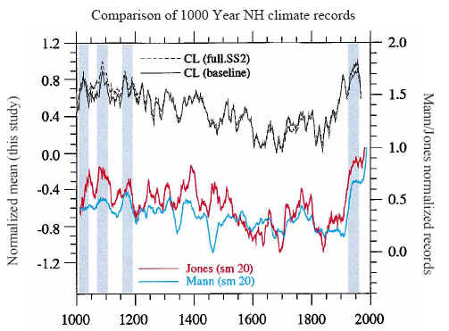
Figure 1. Original Caption to Crowley and Lowery [2000] Figure 2. Comparison of hemispheric composites from this study with that of Jones et al. (9) and Mann et al. (10). Shaded intervals refer to times of peak warmth (see text). The dotted line indicates hemispheric composite values if two lower resolution records [Michigan pollen record (16) and Sargasso Sea d18O record(17)] are added to the baseline composite (see text). All records have been scaled between 0 and 1.

The data for the above figure was never archived. After about 26 emails and nearly 10 months, Crowley provided by email a smoothed version of the underlying data. Figure 2 below was drawn from the email dataset: the black solid and dashed lines replicate the Ambio figure to all intents and purposes. The red line shows values from 1983-1987, indicating that the original CL00 figure ended in 1982, after which date there were only 2 proxies. The availability of the underlying data declined sharply in the 1980s: there were only 5 series in 1982; then only 2 (!) in 1983 – Polar Urals and Dunde, a couple of series on which I’ve written a lot. The Polar Urals version in the dataset ended in 1985 and the Dunde version in 1987 – perhaps as a result of the smoothing methodologies, leaving 0 proxies after from 1988 on. Some of you may recall Crowley’s claims at the UCAR conference that he’s inspected "his" proxies after 1980, claiming that they unequivocably demonstrate warming. It wouldn’t have taken him much time to inspect the two series up to 1987.

Figure 2. Emulation of Figure 2 of Crowley and Lowery [2000]. Dashed “€œ 15 proxy composite; solid black “€œ 13 “€œproxy composite; red- last 5 years (ending 1987) with only 1-2 proxies (used in Briffa et al spaghetti diagram.)

There are a number of issues concerning data quality control, which I do not address here, because of the lack of original data and the desire to illustrate other points. For example, CL2000 appears to use needlessly obsolete versions of some series e.g. the C England documentary series used in CL2000 ends in the early 20th century; the China phenology series of Chu/Zhu [1973] appears to be based on incorrect calendar information according to Zhang [1994].

Crowley and Lowery [2000] stated that the proxy composites were converted to temperature (CL00 Figure 4) by scaling to the Jones CRU series during the periods 1856-1880 and 1920-1965, with the middle period excluded due to low relationship to actual records. Figuring out how they did this has not been easy: I’ll come back to this after discussing data in Crowley [2000].

Crowley [2000]
Crowley [2000] applies Crowley and Lowery [2000] and this time there is a data archive, although not very clear. There are two different figures (Figures 1, 4) in Crowley [2000], which show two different versions of his reconstruction, which has taken me an inordinate amount of time to decode.

The top panel of Crowley [2000] Figure 4 is shown below. Shown in red is version CL2 (which is also provided digitally at WDCP). CL2 is a linear transformation of the "baseline" version in CL00, using 13 proxies; this was relatively easy to confirm. What was less easy to figure out was the procedure for the linear transformation. This was described as scaling of the Ambio series against the CRU temperature in the calibration period of c(1856:1880,1920:1965). (This odd selection was rationalized because of a poor out-of-period match. See below), described as follows:

The two composites were scaled to agree with the Jones et al. (31) instrumental record for the Northern Hemisphere over the intervals 1856-1880 and 1920-1965 (too few of the proxies record information after this date).

The "scaling" is not a "scaling" as understood in recent literature where means and standard deviations are equalized between target and proxy. Here the scaling appears to have (almost certainly) been done by regressing the CRU series against the Ambio-2 series in the calibration period of c(1856:1880,1920:1965). When I did so using the current CRU dataset, I got linear transformation coefficients of (-0.68,1.22) which were quite close to the coefficients of the observed linear transformation (-0.60,1.15) and were very different from any scaling which involves equating standard deviations. The CRU instrumental version used in CL00 is no longer available and the difference in coefficients undoubtedly relates to differences in the instrumental version.

Figure 3. Top Panel – Top panel of Figure 4 from Crowley [2000].; bottom panel (emulation) – black – CL2.Jnsm11; red – CL2; blue – smoothed version of CRU re-centered to 1902-1980 to match MBH.

In passing, Crowley does not appear to do have done many usual statistical tests for the validity of this regression. The first test in any statistics is to plot the residuals, which I’ve done in Figure 3 below, with the black vertical lines denoting the calibration period. The cross-validation R2 for the out-of-calibration (1851:1860,1881:1919;1966:1980) data is 0.005, obviously insignificant (RE: 0.09). The Durbin-Watson statistic is 1.3, well below the required minimum of 1.5. Here’s something else that’s very interesting to me (and providing some dividends from my consideration of ARMA(1,1) processes last summer, which I discussed on the blog.) The Durbin-Watson test considers the residuals from the point of view of an AR1 process – it’s a pretty primitive test. With an AR1 process, the AR1 coefficient was 0.32 (se: 0.0813) and log-likelihood 24.94. However, with an ARMA(1,1) process, the fit was much better (!) with the following coefficients, AR1 0.9565 (se 0.0364) ; MA1 -0.8015 (se 0.0698) and log-likelihood of 33.06. The ARMA(1,1) coefficients have a near-integrated AR1 coefficient, fitting this regression into the spurious regression mould of Deng [2005], with the error-generating process of Perron [1994]. This extremely high AR1 coefficient puts this right into spurious regression territory. As discussed by Deng [2005] and Perron [1994], these sorts of "almost-white almost-integrated" noise can be tricky and hard to spot even with good statistical testing (much less the neolithic or non-statistics of Crowley).

Figure 4. Red-CRU; black – Crowley Index CL2. Calibration done in periods 1861:1880 and 1920:1965.

The Remarkable Instrumental "Splice"

Crowley observed the poor performance of his index in the late 19th century.

The reason for restricting the comparison to these two intervals involves the considerable deviation of the proxy time series from the instrumental record over the interval 1880″€œ1920 (Fig. 4). The deviation occurs in 5 of our records (White Mountains, Colorado, Urals, and west and east China records), has been observed before (10, 33) and been attributed to (10) anomalous tree-ring growth due to the late 19th century rise in CO2. Mann et al. (10) addressed this problem by removing the postulated CO2 growth effect before estimating past temperatures. However, because this response also occurs in the Chinese phenological data set, another source of variance for high tree-ring growth rates cannot be excluded.

So for his final construction, Crowley carried out the following remarkable steps, in which he spliced the CRU data into his proxy index. We’ll start with Figure 1 of Crowley [2000] shown below:

Figure 5. Original Caption to Crowley [2000] Fig. 1. Comparison of decadally smoothed Northern Hemisphere mean annual temperature records for the past millennium (1000-1993), based on reconstructions of Mann et al. (Mn) (11) and CL (12). The latter record has been spliced into the 11-point smoothed instrumental record (16) in the interval in which they overlap. CL2 refers to a new splice that gives a slightly better fit than the original (12). The autocorrelation of the raw Mann et al. time series has been used to adjust (adj) the standard deviation units for the reduction in variance on decadal scales.

In the Figure 1 dataset at WDCP, the series CL2 (not illustated in the Figure) is the linear transformation of the Ambio-13 series version, except that it is terminated in 1965, rather than 1982. Crowley says that it ends early because of reduced proxy coverage, but it also goes down. The series CL2.Jns11 is identical to the series CL2 from 1000-1870, but differs from 1871-1993. It looks like a 11-point smooth of the CRU dataset from 1871-1993 is spliced to CL2 from 1000-1870 to make the series CL2.Jns11 in Figure 1.

The Figure 4 dataset at WDCP had another puzzle. Figure 4 CL2.Jnsm11 is identical to the Figure 1 CL2.Jnsm11 version. It also contains a series CL2.Jns11 adjusted, which puzzled me for a long time. It is identical to Figure 4 CL2Jns11 (the splice of Ambio and instrumental data) except from 1871-1965. Here the CL2 data is re-substituted back into the CL2.Jnsm11 series for the period 1871-1965. So it is CL2 spliced with instrumental data from 1966 on.

Returning now to Crowley [2000] Figure 1, the series CL2.Jns (11) is the CL2 data up to 1870 and then is the CRU instrumental data to 1993 ( which reflects values up to 1998 due to smoothing). The MBH versions illustrated also splice reconstruction and instrumental values. Thus, Crowley made two different splices of the temperature record into the proxy record. One splice is made in 1965, with proxy values for the 13-site composite (see below) before 1965 and instrumental values from 1965 to 1998 (with the 11-point smooth version ending in 1993). A second version is spliced in 1870, with proxy values from the 13-site composite before 1870 and instrumental records after wards.

A final observation on this: none of the archived versions of Crowley-Lowery at WDCP contains the proxy data past 1965. These versions all contain splices of one form or another. Because the reconstruction is a linear transformation of the Ambio data, it can be derived to 1982 from the Ambio data, but not otherwise.

I will discuss an interesting comment of Mann’s about splicing of the instrumental record tomorrow. I’ll also look at a version archived at Briffa, which may embody the unspliced version.