Marcott’s Dimple: A Centering Artifact

One of the longstanding CA criticisms of paleoclimate articles is that scientists with little-to-negligible statistical expertise too frequently use ad hoc and homemade methods in important applied articles, rather than proving their methodology in applied statistical literature using examples other than the one that they’re trying to prove.

Marcott’s uncertainty calculation is merely the most recent example. Although Marcott et al spend considerable time and energy on their calculation of uncertainties, I was unable to locate a single relevant statistical reference either in the article or the SI (nor indeed a statistical reference of any kind.) They purported to estimate uncertainty through simulations, but simulations in the absence of a theoretical framework can easily fail to simulate essential elements of uncertainty. For example, Marcott et al state of their simulations: “Added noise was not autocorrelated either temporally or spatially.” Well, one thing we know about residuals in proxy data is that they are highly autocorrelated both temporally and spatially.

Roman’s post drew attention to one such neglected aspect.

Very early in discussion of Marcott, several readers questioned how Marcott “uncertainty” in the mid-Holocene could possibly be lower than uncertainty in recent centuries. In my opinion, the readers are 1000% correct in questioning this supposed conclusion. It is the sort of question that peer reviewers ought to have asked. The effect is shown below (here uncertainties are shown for the Grid5x5 GLB reconstruction) – notice the mid-Holocene dimple of low uncertainty. How on earth could an uncertainty “dimple” arise in the mid-Holocene?

uncertainty
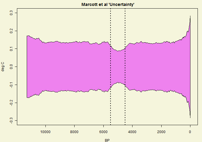
Figure 1. “Uncertainty” from Marcott et al 2013 spreadsheet sheet 2. Their Figure 1 plot results with “1 sigma uncertainty”.

It seems certain to me that “uncertainty” dimple is an artifact of their centering methodology, rather than of the data.

Marcott et al began their algorithm by centering all series between BP4500 and BP5500 – these boundaries are shown as dotted lines in the above graphic. The dimple of low “uncertainty” corresponds exactly to the centering period. It has no relationship to the data.

Arbitrary re-centering and re-scaling is embedded so deeply in paleoclimate that none of the practitioners even seem to notice that it is a statistical procedure with inherent estimation issues. In real statistics, much attention is paid to taking means and estimating standard deviation. The difference between modern (in some sense) and mid-Holocene mean values for individual proxies seems to me to be perhaps the most critical information for estimating the difference between modern and mid-Holocene temperatures, but, in effect, Marcott et al threw out this information by centering all data on the mid-Holocene.

Having thrown out this information, they then have to link their weighted average series to modern temperatures. They did this by a second re-centering, this time adjusting the mean of their reconstruction over 500-1450 to the mean of one of the Mann variations over 500-1450. (There are a number of potential choices for this re-centering, not all of which yield the same rhetorical impression, as Jean S has already observed.) That the level of the Marcott reconstruction should match the level of the Mann reconstruction over 500-1450 proves nothing: they match by construction.

The graphic shown above – by itself – shows that something is “wrong” in their estimation of uncertainty – as CA readers had surmised almost immediately. People like Marcott are far too quick to presume that “proxies” are a signal plus simple noise. But that’s not what one actually encounters: the difficulty in the field is that proxies all too often give inconsistent information. Assessing realistic uncertainties in the presence of inconsistent information is a very non-trivial statistical problem – one that Marcott et al, having taken a wrong turn somewhere, did not even begin to deal with.

I’m a bit tired of ad hoc and homemade methodologies being advanced by non-specialists in important journals without being established in applied statistical journals. We’ve seen this with the Mannian corpus. Marcott et al make matters worse by failing to publish the code for their novel methodology so that interested readers can quickly and efficiently see what they did, rather than try to guess at what they did.

While assembling Holocene proxies on a consistent basis seems a useful bit of clerical work, I see no purpose in publishing an uncertainty methodology that contains such an obvious bogus artifact as the mid-Holocene dimple shown above.

The Quelccaya Update

Lonnie Thompson has done a much better job of archiving data for his recent update Quelccaya – see NOAA here – both in terms of information and promptness.

Quelccaya is familiar territory for Thompson as it was the location of his first tropical ice cores (1983) and his first publication of this type. Thompson published a first update of Quelccaya d18O values in 2006 (PNAS) but only 5-year average data and only to the late 1990s. The new dataset gives annual data (previously available from the 1983 cores from 470 to 1983) from 226 to 2009.

Below is a graphic showing twentieth century on, comparing to the PNAS 2006 five-year data. The extension covers the big 1998-99 El Nino with a dotted red line. Since 1998-99 is known to be an exceptionally warm year, it is interesting to observe that it is manifested at Quelccaya as an negative downspike.

2013-twentieth

There has been a longstanding dispute about whether d18O at Quelccaya and other tropical glaciers is a proxy for temperature or for the amount of precipitation. In monsoon region precipitation, negative d18O values show rain-out. Quelccaya d18O has been (IMO plausibly) interpreted by Hughen as evidence of north-south migration of the ITCZ, with Hughen comparing Quelccaya information particularly to information from Cariaco, Venezuela.

It seems to me that, among specialists, Thompson is probably standing fairly alone in claiming that d18O at tropical glaciers is a proxy for temperature rather than amount effect. (Because of Thompson’s eminence, the contradiction of his results is mostly implied, rather than directly stated.) Despite these reservations among specialists, Thompson’s d18O records have been widely cited by Mann and other multiproxy jockeys (both directly and through the Yang composite) and are important contributors to some of the AR4 Hockey Sticks. “Dr Thompson’s Thermometer” was proclaimed in Inconvenient Truth as supposedly vindicating the Mann Hockey Stick, although the graphic shown in AIT was merely the Mann hockey stick wearing whiskers, so naturally it confirmed itself.

Because the 1998 El Nino was so big, it provides a good test case for temperature vs amount. It seems to me that the negative downspike for the big 1998 El Nino is decisive against Thompson.

The PNAS version of the data left off showing a sort of uptick. The extension to 2009 does not seem to me to be going off the charts.

Update Apr 8. here is a comparison of Quelccaya O18 to HadCRU GLB (both scaled over the 20th century). I’ve used GLB because Quelccaya is used to deduce global temperatures in multiproxy studies, not temperatures at Cuzco. Quelccaya O18 values obviously do not capture the temperature trend. Marcott/Mann defenders say that we don’t need proxies to know that temperature has gone up in the 20th century. Quite so. Quelccaya was not a Marcott proxy, but it was important in Mann et al 2008 and other multiproxy reconstructions. What does this sort of thing really tell us?

quelc-vs-had

Anthony’s coverage of the release of this data prompted some discussion of the Thompsons as serial non-archivers, referring to my post here. It is worth commending Thompson for prompt archiving of the present data, but that does not refute past criticism of both Ellen and Lonnie. (I note that Thompson has mitigated some of that criticism by archiving some data on old cores, even within the past year.)

The post in question actually was directed at Ellen Mosley-Thompson, who, as far as I can tell, has not archived a single data set in which she was lead PI in over 30 years in the business. I stated the following:

She has spent her entire career in the ice core business> According to her CV, she has led “nine expeditions to Antarctica and six to Greenland to retrieve ice cores”. However, a search of the NOAA paleo archive for data archived by Ellen Mosley-Thompson shows only one data set from Antarctica or Greenland associated with her. Lest this example be taken to mar her otherwise unblemished record of non-archiving, the data was published in 1981 while she was still junior and, according to its readme, it was transcribed by a third party and contributed in her name. I believe that it’s fair that she has not archived at NOAA (or, to my knowledge, elsewhere) any data from the “nine expeditions to Antarctica and six to Greenland”.

I did a fairly thorough review of Thompson’s non-archiving as of July 2012 here. Nick Stokes at WUWT claimed that my posts were refuted by his being able to locate Thompson data at NOAA. Unfortunately, this is the sort of misdirection that is all too prevalent in the field.

I am obviously aware of the NOAA archive. While, like anyone else, I make my share of mistakes, the odds of me being wrong in the trivial way that Stokes asserted are negligible. While Ellen is listed as a co-contributor on expeditions led by Lonnie, the above statement is true as written.

Nor does Nick’s location of NOAA archives (which I know intimately) refute my criticisms of Thompson’s archive here. The Lonnie situation is much less bad than when I started criticizing him: when I first got interested, no data for Dunde, Guliya or Dasuopu had been archived and Thompson blew off requests for data. Matters are less bad, but still very unsatisfactory. Inconsistent grey versions of Dunde and other series are in circulation. This can only be sorted out by archiving all samples together with dating criteria. I’ve characterized such an archive as Thompson’s legacy – something that he should be proud of and not resist.

I’ve also strongly criticized Thompson’s failure to archive the Bona-Churchill data, sampled long before the recent Quelccaya data. This data was already overdue in 2006, when I first criticized its non-publication and non-archiving. At the time, I observed (somewhat acidly, I’ll admit) that if the data had a big upspike in the late 20th century, Thompson would have press released and published. Because the dog didn’t bark, I predicted that the data went the “wrong” way. Seven years later, Thompson still hasn’t published Bon-Churchill, though results were shown at a workshop a number of years ago, showing that they did indeed go the ‘wrong” way, as I had surmised.

My Prediction for dO18 at Bona Churchill

Gleanings on Bona Churchill


https://climateaudit.org/tag/bona-churchill/

Marcott Monte Carlo

So far, the focus of the discussion of the Marcott et al paper has been on the manipulation of core dates and their effect on the uptick at the recent end of the reconstruction. Apologists such as “Racehorse” Nick have been treating the earlier portion as a given. The reconstruction shows that mean global temperature stayed pretty much constant varying from one twenty year period to the next by a maximum of .02 degrees for almost 10000 years before starting to oscillate a bit in the 6th century and then with a greater amplitude beginning about 500 years ago. The standard errors of this reconstruction range from a minimum of .09 C (can this set of proxies realistically tell us the mean Temperature more than 5 millennia back within .18 degrees with 95% confidence?) to a maximum of .28 C. So how can they achieve such precision?

Twenty year reconstruction changes

The Marcott reconstruction uses a methodology generally known as Monte Carlo. In this application, they supposedly account for the uncertainty of the proxy by perturbing both the temperature indicated by each proxy value as well as the published time of observation. For each proxy sequence, the perturbed values are then made into a continuous series by “connecting the dots” with straight lines (you don’t suppose that this might smooth each series considerably?) and the results from this are recorded for the proxy at 20 year intervals. In this way, they create 1000 gridded replications of each of their 73 original proxies. This is followed up with recalculating all of the “temperatures” as anomalies over a specific 1000 period (where do you think you might see a standard error of .09?). Each of the 1000 sets of 73 gridded anomalies is then averaged to form 1000 individual “reconstructions”. The latter can be combined in various ways and from this set the uncertainty estimates will also be calculated.

The issue I would like to look at is how the temperature randomization is carried out for certain classes of proxies. From the Supplementary Information:

Uncertainty

We consider two sources of uncertainty in the paleoclimate data: proxy-to-temperature calibration (which is generally larger than proxy analytical reproducibility) and age uncertainty. We combined both types of uncertainty while generating 1000 Monte Carlo realizations of each record.

Proxy temperature calibrations were varied in normal distributions defined by their 1σ uncertainty. Added noise was not autocorrelated either temporally or spatially.

a. Mg/Ca from Planktonic Foraminifera – The form of the Mg/Ca-based temperature proxy is either exponential or linear:
Mg/Ca = (B±b)*exp((A±a)*T)
Mg/Ca =(B±b)*T – (A±a)
where T=temperature.
For each Mg/Ca record we applied the calibration that was used by the original authors. The uncertainty was added to the “A” and “B” coefficients (1σ “a” and “b”) following a random draw from a normal distribution.

b. UK’37 from Alkenones – We applied the calibration of Müller et al. (3) and its uncertainties of slope and intercept.
UK’37 = T*(0.033 ± 0.0001) + (0.044 ± 0.016)

These two proxy types account for (19 (Mg/Ca) and 31 (UK’37)) 68% of the proxies used by Marcott et al. Any missteps in how these are processed would have a very substantial effect on the calculated reconstructions and error bounds. Both of them use the same type of temperature randomization so we will examine only the Alkenone series in detail.

The methodology for converting proxy values to temperature comes from a (paywalled) paper: P. J. Müller, G. Kirst, G. Ruthland, I. von Storch, A. Rosell-Melé, Calibration of the alkenone 497 paleotemperature index UK’37 based on core-tops from the eastern South Atlantic and the 498 global ocean (60N-60S). Geochimica et Cosmochimica Acta 62, 1757 (1998). Some information on Alkenones can be found here.

Müller et al use simple regression to derive a single linear function for “predicting” proxy values from the sea surface temperature:

UK’37 = (0.044 ± 0.016) + (0.033 ± 0.001)* Temp

The first number in each pair of parentheses is the coefficient value, the second is the standard error of that coefficient. You may notice that the standard error for the slope of the line in the Marcott SI is in error (presumably typographical) by a factor of 10. These standard errors have been calculated from the Müller proxy fitting process and are independent of the Alkenone proxies used by Marcott (except possibly by accident if some of the same proxies have also been used by Marcott). The relatively low standard errors (particularly of the slope) are due to the large number of proxies used in deriving the equation.

According to the printed description in the SI, the equation is applied as follows to create a perturbed temperature value:

UK’37 = (0.044 + A) + (0.033 + B)* Pert(Temp)

[Update: It has been pointed by faustusnotes at Tamino’s Open mind that certain values that I had mistakenly interpreted as standard errors were instead 95% confidence limits. The changes in the calculations below reflect the fact the the correct standard deviations are approximate half of those amounts: 0.008 and 0.0005.]

where A and B are random normal variates generated from independent normal distributions with standard deviations of 0.016 0.008 and 0.001 0.0005, respectively.

Inverting the equation to solve for the perturbed temperature gives

Pert(Temp) = (UK’37 – 0.044)/(0.033 + B) – A / (0.033 + B)

If we ignore the effect of B (which in most cases would have a magnitude no greater than .003), we see that the end result is to shift the previously calculated temperature by a randomly generated normal variate with mean 0 and standard deviation equal to 0.016/0.033 = .48 0.008/0.033 = 0.24. In more than 99% of the cases this shift will be less than 3 SDs or about 1.5 0.72 degrees.

So what can be wrong with this? Well, suppose that Müller had used an even larger set of proxies for determining the calibration equation, so large that both of the coefficient standard errors became negligible. In that case, this procedure would produce an amount of temperature shift that would be virtually zero for every proxy value in every Alkenone sequence. If there was no time perturbation, we would end up with 1000 almost identical replications of each of the Alkenone time series. The error bar contribution from the Alkenones would spuriously shrink towards zero as well.

What Marcott does not seem to realize is that their perturbation methodology left out the most important uncertainty element in the entire process. The regression equation is not an exact predictor of the the proxy value. It merely represents the mean value of all proxies at a given temperature. Even if the coefficients were known exactly, the variation of the individual proxy around that mean would still produce uncertainty in its use. The randomization equation that they should be starting with is somewhat different:

UK’37 = (0.044 + A) + (0.033 + B)* Pert(Temp) + E

where E is also a random variable independent of A and B and with standard deviation of the predicted proxy equal to 0.050 obtained from the regression in Müller:

The perturbed temperature now becomes

Pert(Temp) = (UK’37 – 0.044)/(0.033 + B) – (A + E) / (0.033 + B)

and again ignoring the effect of B, the new result is equivalent to shifting the temperature by a single randomly generated normal variate with mean 0 and standard deviation given by

SD = sqrt( (0.016/0.033)2 + (0.050/0.033)2 ) = 1.59
SD = sqrt( (0.008/0.033)2 + (0.050/0.033)2 ) = 1.53

The variability of the perturbation is now three 6.24 times as large as that calculated when only the uncertainties in the equation coefficients are taken into account. Because of this, the error bars would increase substantially as well. The same problem would occur for the Mg/Ca proxies as well, although the magnitudes of the increase in variability would be different. In my opinion, this is a possible problem that needs to be addressed by the authors of the paper.

The regression plot and the residual plot from Müller give an interesting view of what the relationship looks like.

I would also like someone to tell me if the description for ice cores means what I think it means:

f. Ice core – We conservatively assumed an uncertainty of ±30% of the temperature anomaly (1σ).

If so, …

Tom Curtis Writes

While CA readers may disagree with Tom Curtis, we’ve also noticed that he is straightforward. Recently, in comments responding to my recent post on misrepresentations by Lewandowsky and Cook, Curtis agreed that “Lewandowsky’s new addition to his paper is silly beyond belief”, but argued that “the FOI data does not show Cook to have lied about what he found. He was incorrect in his claims about where the survey was posted; but that is likely to be the result of faulty memory.”

Showing both integrity and personal courage, Curtis has sent me the email published below (also giving me permission to publish the excerpt shown.) While Curtis agreed that Cook’s statement to Chambers could not possibly be true, Curtis re-iterates his belief that Cook is honest, though he is obviously troubled by the incident. Curtis also reports that, as early as last September, he emailed both Lewandowsky (cc Oberauer) and Cook informing them that no link to the Lewandowsky survey had been posted at the SKS blog, only a tweet – a warning inexplicably ignored by Lewandowsky and Oberauer in their revisions to Lewandowsky et al (Psych Science). Continue reading

April Fools’ Day for Marcott et al

Q. Why did realclimate publish the Marcott FAQ on Easter Sunday?
A. Because if they’d waited until Monday, everyone would have thought it was an April Fools’ joke. Continue reading

The Marcott Filibuster

Marcott et al have posted their long-promised FAQ at realclimate here. Without providing any links to or citation of Climate Audit, they now concede:

20th century portion of our paleotemperature stack is not statistically robust, cannot be considered representative of global temperature changes, and therefore is not the basis of any of our conclusions.

Otherwise, their response is pretty much a filibuster, running the clock on questions that have not actually been asked and certainly not at issue by critics. For questions and issues that I’ve actually raised, for the most part, they merely re-iterate what they already said. Nothing worth waiting for. Continue reading

Aging as a State of Mind

Bobbie Hasselbring, editor of Real Food Traveller, has an article on “Aging as a State of Mind”. Her article concludes as follows:

Katherine McIntyre is 89 years old. She’s the oldest person ever to have zip lined at High Life Adventures. She’s a working travel journalist. And she kept me from even wondering whether I’m afraid of heights. And, you know what? I’m not afraid. Because Katherine isn’t afraid and she’s one of my heroes.

Mine as well.

Lewandowsky Doubles Down

Last fall, Geoff Chambers and Barry Woods established beyond a shadow of a doubt that no blog post linking to the Lewandowsky survey had ever been published at the Skeptical Science (SKS) blog. Chambers reasonably suggested at the time that the authors correct the claim in the article to reflect the lack of any link at the SKS blog. I reviewed the then available information on this incident in September 2012 here.

Since then, information obtained through FOI by Simon Turnill has shown that responses by both Lewandowsky and Cook to questions from Chambers and Woods were untrue. Actually, “untrue” does not really do justice to the measure of untruthfulness, as the FOI correspondence shows that the untruthful answers were given deliberately and intentionally. Chambers, in a post entitled Lewandowsky the Liar, minced no words in calling Lewandowsky “a liar, a fool, a charlatan and a fraud.”

Even though the untruthfulness of Lewandowsky and Cook’s stories had been clearly demonstrated by Geoff Chambers in a series of blog articles (e.g. here), in the published version of the Hoax paper, instead of correcting prior untrue claims about SKS, Lewandowsky doubled down, repeating and substantially amplifying the untrue claim. Continue reading

Bent Their Core Tops In

In today’s post, I’m going to show Marcott-Shakun redating in several relevant cases. The problem, as I’ve said on numerous occasions, has nothing to do with the very slight recalibration of radiocarbon dates from CALIB 6.0.1 (essentially negligible in the modern period in discussion here), but with Marcott-Shakun core top redating. Continue reading

Hiding the Decline: MD01-2421

As noted in my previous post, Marcott, Shakun, Clark and Mix disappeared two alkenone cores from the 1940 population, both of which were highly negative. In addition, they made some surprising additions to the 1940 population, including three cores whose coretops were dated by competent specialists 500-1000 years earlier.

While the article says that ages were recalibrated with CALIB6.0.1, the differences between CALIB6.0.1 and previous radiocarbon calibrations is not material to the coretop dating issues being discussed here. Further, Marcott’s thesis used CALIB6.0.1, but had very different coretop dates. Marcott et al stated in their SI that “Core tops are assumed to be 1950 AD unless otherwise indicated in original publication”. This is not the procedure that I’ve observed in the data. Precisely what they’ve done is still unclear, but it’s something different.

In today’s post, I’ll examine their proxy #23, an alkenone series of Isono et al 2009. This series is a composite of a piston core (MD01-2421), a gravity core (KR02-06 St. A GC) and a box/multiple core (KR02-06 St A MC1), all taken at the same location. Piston cores are used for deep time, but lose the top portion of the core. Coretops of piston cores can be hundreds or even a few thousand years old. Box cores are shallow cores and the presently preferred technique for recovering up-to-date results.

There are vanishingly few alkenone series where there is a high-resolution box core accompanying Holocene data. Indeed, within the entire Marcott corpus of ocean cores, the MD01-241/KNR02-06 splice is unique in being dated nearly to the present. Its published end date was -41BP (1991AD). Convincing support for modern dating of the top part of the box core is the presence of a bomb spike:

A sample from 3 cm depth in the MC core showed a bomb spike. The high sedimentation rate (average 31 cm/ka) over the last 7000 years permits analysis at multidecade resolution with an average sample spacing of ~32 years.

Despite this evidence for modern sediments, Marcott et al blanked out the top three measurements as shown below:

md01-2421 excerpt
Table 1. Excerpt from Marcott et al spreadsheet

By blanking out the three most recent values of their proxy #23, the earliest dated value was 10.93 BP (1939.07 AD). As a result, the MD01-2421+KNR02-06 alkenone series was excluded from the 1940 population. I am unable to locate any documented methodology that would lead to the blanking out of the last three values of this dataset. Nor am I presently aware of any rational basis for excluding the three most recent values.

Since this series was strongly negative in the 20th century, its removal (together with the related removal of OCE326-GGC30 and the importation of medieval data) led to the closing uptick.

BTW in the original publication, Isono et al 2009 reported a decrease in SST from Holocene to modern times that is much larger than the Marcott NHX estimate of less than 1 deg C, reporting as follows:

the SST decreased by ~5 °C to the present (16.7 °C), with high-frequency variations of ~1 °C amplitude (Fig. 2).

A plot of this series is shown below, with the “present” value reported by Isono et al shown as a red dot.

MD03-2421 splice