JDOhio: Was Michael Mann Exonerated by the Post-Climategate Investigations as Was Decided by the DC Court of Appeals?

SM: This article by JD Ohio was submitted and briefly online on February 23, 2018, but, for some reason that I don’t recall, was taken offline. In any event, as Mann’s ancient libel case wends its way into a DC court, I noticed that it was still pending.  It deals concisely with a central issue in the case. 

By JDOhio

Analysis of Court of Appeals’ Defamation Opinion Holding That
Climategate Inquiries Exonerated Michael Mann

Foreword

I have followed climate matters for a long time and have been aware of the inquiries that followed Climategate. So, instinctively, when Michael Mann claimed that Climategate inquiries exonerated him, I believed the claim was incorrect. There were four inquiries that the appellate Court focused on (See p. 96 of court opinion which referred to “four separate investigations”) which accepted Mann’s argument that he had been exonerated. See link to opinion: https://cei.org/litigation/michael-e-mann-v-national-review-and-cei-et-al The Court’s identification of the inquiries was confusing, but I will focus on the main reports that seem to be the basis for the Court’s conclusion. Having reviewed the inquiries closely, my opinion is still that the investigations did not exonerate Mann.

Some of the emails are misleading, and the various reports and graphs that are important to the resolution of this case are very hard to keep track of. If one attempts to dive in the middle of this dispute without having a clear idea of the background, it is easy to get sucked down a rathole of confusing and overlapping studies, graphs, emails and inquiries. The point of this blog post is to create an accurate reference work that is comparatively easy to follow. So, although it is somewhat tedious, I have gone into a good amount of detail on what would otherwise be minor details.

Concise Summary of Findings

Although the Court was not always clear as to what four studies it was looking at (See *** at end of this post), here is a brief description of my findings pertaining to the studies most relevant to the Court opinion.

1. Muir Russell Report (also called called the Independent Climate Change E-mails Review (ICCER): This report was commissioned by the University of East Anglia (UEA) to look at issues that arose concerning the UEA following the release of 1073 UEA emails. Although Mann was mentioned in some of the emails, the real focus was on the academic integrity of the UEA. It could not exonerate Mann. The House of Commons reviewed Muir Russell, and the Court subsumed Muir Russell under the United Kingdom House of Commons Report.

2. Oxburgh Report (formally known as the “Science Appraisal Panel of Climatic Research Unit of University of East Anglia): This report was reviewed by the House of Commons report. It didn’t even mention Mann or any of his publications.

3. Penn State Two Stage Inquiry: These reports did not closely examine scientific criticism of Mann’s work, and Penn State totally flubbed the investigation into whether, at the very least, Mann indirectly took part in an email deletion scheme when he forwarded an email from Phil Jones to Gene Wahl asking for the deletion of emails pertaining to the Fourth Assessment Report (AR4) of the IPCC.

4. National Science Foundation (NSF) Close-Out Memo regarding Penn State investigation of Michael Mann. This Memo is completely unsubstantiated; it is not clear who wrote the memo or did the underlying work. Also, although it is widely believed that it is referring to Penn State and Mann, it never explicitly names either.

5. EPA Reconsideration of Endangerment Finding: On p. 83 of the opinion, the Court referred to the EPA as having found that the science underlying the Hockey Stick was valid. When the EPA did look at Mann specifically, it downplayed his contributions, and he was only mentioned once in the Reconsideration Report. (See p. 85 of report) Since the EPA’s consideration of Mann was so skimpy, and was only briefly mentioned by the Court, I will not discuss it further.

Overview of Important Science and Email Issues
Useful to Understanding the Legal Dispute

I. Problems with Tree Proxies (Divergence)

Around 1960, tree proxies which seemed to be accurate indicators of rising and falling temperatures began showing declines (less growth and density), when the instrumental records were showing rising temperatures. There seems to be no doubt that a number of tree proxies were simply inaccurate after 1960. See https://climateaudit.org/2008/11/30/criag-loehle-on-the-divergence-problem/ Thus, to the extent that tree proxies were known to be inaccurate it is sometimes reasonable, with full DISCLOSURE, to splice together old tree proxies from, say 500 years ago up to 1960 with instrumental records. If you continued with tree proxies known to be defective, it would obviously be wrong.

The problem with tree proxies raises a huge issue. If they aren’t accurate now, how do we know that they were accurate four or eight hundred years ago? The answer is that we don’t know. However, for some reason, a lot of skeptics place the vast majority of their focus on the instrumental temperatures and not the fairly easy question dealing with the apparent unreliability of proxies. It seems to me that the only way anyone can say that today’s global average temperatures (for example) are, let’s say 2.5 degrees C higher than those in the 10th century is to preface that statement with the qualifier, my best guess is….

II. The Misleading “Hide the Decline” Email

From Phil Jones: “I’ve just completed Mike’s [Mann’s] Nature trick of adding in the real temps to each series for the last 20 years (i.e., from 1981 onwards) and from 1961 for Keith’s to hide the decline.”

From: Phil Jones [November 1999]
To: ray bradley ,mann@xxxxx.xxx, mhughes@xxxx.xxx
Subject: Diagram for WMO Statement
Date: Tue, 16 Nov 1999 13:31:15 +0000
Cc: k.briffa@xxx.xx.xx,t.osborn@xxxx.xxx

Dear Ray, Mike and Malcolm,
Once Tim’s got a diagram here we’ll send that either later today or
first thing tomorrow.
I’ve just completed Mike’s Nature trick of adding in the real temps
to each series for the last 20 years (ie from 1981 onwards) amd from
1961 for Keith’s to hide the decline. Mike’s series got the annual
land and marine values while the other two got April-Sept for NH land
N of 20N. The latter two are real for 1999, while the estimate for 1999
for NH combined is +0.44C wrt 61-90. The Global estimate for 1999 with
data through Oct is +0.35C cf. 0.57 for 1998.
Thanks for the comments, Ray.

Cheers
Phil

Prof. Phil Jones
Climatic Research Unit Telephone +44 (0) xxxxx
School of Environmental Sciences Fax +44 (0) xxxx
University of East Anglia
Norwich Email p.jones@xxxx.xxx
See https://climateaudit.org/2009/11/20/mike%e2%80%99s-nature-trick/

(See also Climate Audit https://climateaudit.org/2011/03/29/keiths-science-trick-mikes-nature-trick-and-phils-combo/)

When you first hear the phrase “hide the decline,” it is easy to believe that the speaker is talking about hiding a real decline in instrumental temperatures. Instead what Jones is talking about is hiding the decline evident in tree proxies after approximately 1960. However, if you are going to attempt to have 1,000 year or 1,400 year temperature reconstructions, just a little bit of thought will make it clear that the tree ring proxies have to be dropped after 1960. On the other hand, there is a large question as to whether it is worthwhile to do 1000 year reconstructions when the proxies used are known to be unreliable in today’s world; how is it really possible to know that proxies were reliable 1000 years ago?

It is true that before the 1998 Hockey Stick introduced by Mann, the divergence problem had been discussed in was openly discussed in the literature. What Jones was doing when he spoke of “hide[ing] the decline” was attempting to gloss over the divergence problem and the decline in temperatures that would be shown by continuing to use tree proxies when extrapolating temperatures as shown in a paper written by Keith Briffa of University of East Anglia [UEA] who was part of the Climatic Research Unit (CRU).

III. Mike’s Nature Trick

This Trick is mentioned in the Nov. 16, 1999 email.  To fully understand it, one must understand statistical smoothing and be conversant with, and compare, three different studies.  I am not good at statistics and any explanation I could give would unduly complicate this post.  So, I am skipping it.  Steve McIntyre was kind enough to provide his summary, which is attached at the end of this post.  See ***4

Analysis of “Exoneration” Part of Court of Appeals Decision

The Court of Appeals issued a lengthy, 111 page opinion, holding that Michael Mann had a valid defamation case to present against Rand Simberg, Rich Lowry, the National Review , the Competitive Enterprise Institute, and inferentially, Mark Steyn. (Who did not appeal, but whose case would rise and fall on the case of the others). The portion of the opinion that I am focusing on is that portion, from p. 82 to p. 97 in which the Court heavily relied on four investigations to reach the conclusion that the defendants could have acted with actual malice in criticizing Mann for the research he did.

My basic conclusion is that the four “investigations/endeavors” did not thoroughly investigate Mann and that the Court made a clear mistake when it incorrectly relied on the investigations to allow Mann’s lawsuit to proceed.

A. Some Publications, Resources and Facts That Are Important to the Case.
1. The Court of Appeals Decision
(See https://cei.org/litigation/michael-e-mann-v-national-review-and-cei-et-al )
2. The alleged defamatory columns attached to the end of the decision.
3. The Defendants are not claiming that Mann acted in a criminally fraudulent manner in the sense that he could have made up numbers. The defendants were using the term “fraud” in a polemical sense. In common polemical usage, “fraudulent” doesn’t mean honest-to-goodness criminal fraud. It means intellectually bogus and wrong.” (See p. 110 of the opinion)
4. MBH 98 (first Hockey Stick paper), MBH 99 (Second Hockey Stick Paper, going
1000 years further) See https://en.wikipedia.org/wiki/Michael_E._Mann See also, S. McIntyre collection of Hockey Stick publications.

Hockey Stick Studies


5. WMO Diagram and explanation of Hide the Decline email. Also, IPCC Third Assessment Graph
https://climateaudit.org/2009/12/10/ipcc-and-the-trick/ For more context, see http://www.americanthinker.com/articles/2010/02/climategates_phil_jones_confes.html
6. Hide the Decline email:
I’ve just completed Mike’s Nature trick of adding in the real temps to each series for the last 20 years (i.e., from 1981 onwards) and from 1961 for Keith’s to hide the decline. See:
https://www.justfacts.com/globalwarming.hidethedecline.asp
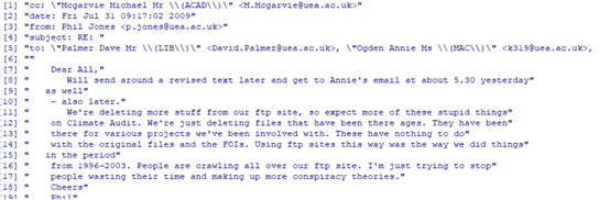
7. Phil Jones deletion email request sent to Mann for him to forward to Eugene Wahl, which Mann did.
“Mike,
Can you delete any emails you may have had with Keith [Briffa] re AR4? Keith will do likewise… Can you also email Gene [Wahl] and get him to do the same? I don’t have his new email address. We will be getting Caspar [Ammann] to do likewise.
Cheers, Phil

**** Mann reply:

“Hi Phil,
… I’ll contact Gene [Wahl] about this ASAP. His new email is: generwahl@xxx talk to you later, mike

For context, see: https://climateaudit.org/2011/02/23/new-light-on-delete-any- emails/ and https://climateaudit.org/2011/09/02/nsf-on-jones- email-destruction-enterprise/

B. Conceptual Errors Made by the Court of Appeals

The Court makes three fundamental errors. First, it assumes that those who label themselves as investigators really do investigate. Second, it assumes that a general investigation (assuming arguendo that a real investigation occurred) into a scientific field of study that finds there was no fraud in the field exonerates all of those in that field even if any individual’s work was only tangentially involved, if at all. Third, it assumes that those with advanced degrees, by virtue of their possession of advanced degrees, are competent and fair commentators and investigators in an area of much controversy. (See p. 85 of opinion)

Although the Court refers to “eight separate inquiries” (p. 82), in reality it only focused on four. The Court concluded on p. 96 that:

“We come to the same conclusion as in Nader. In the case before us now, not
one but four separate investigations were undertaken by different bodies following
accusations, based on the CRU emails, that Dr. Mann had engaged in deceptive
practices and scientific and academic misconduct. Each investigation unanimously
concluded that there was no misconduct.”

For a more detailed explanation of the four reports, one may go to McKitrick. See https://www.bing.com/search?q=ross+mckitrick+summary+of+climategate+investigations&qs=n&form=QBRE&sp=-1&pq=ross+mckitrick+summary+of+climategate+investigations&sc=0-52&sk=&cvid=DCB9DE01989A4284AA5A0D887E2E1254 I will discuss the the two UEA sponsored endeavors first, then the House of Commons report which evaluated them, and then discuss the NSF report.

1. The House of Commons Report

On January 25, 2011, the House of Commons issued its report regarding the investigations of the Climatic Research Unit of the University of East Anglia. Essentially what it did was to evaluate the Oxburgh and Muir Russell Reports. Inferentially, it also independently, in a small way, evaluated climate science as practiced by the CRU.

With respect to Michael Mann, his name is found three times in the report. See https://publications.parliament.uk/pa/cm201011/cmselect/cmsctech/444/44410.htm His name was mentioned twice in connection with two papers he co-authored, and once in regards to an email that Phil Jones sent him asking Mann to keep matters dealing with multi-proxy studies secret as between two other climate research colleagues. (See para. 71 of Report) Although the ethics of Mr. Jones were being examined, there was no focus on ethics of Michael Mann.

There are numerous scientific and practical issues raised by the report. However, although Mann was mentioned tangentially, there was no focus whatsoever on the individual quality of his work or of Mann’s personal ethics.

The report, in a small way, validates climate science by finding that those working at the UEA were not fraudulently manipulating data and were not unethically manipulating peer review. However, it in no way focused on Mann. Thus, there is no way that it exonerated Mann.

2. Oxburgh Endeavor (claimed investigation)

The House of Commons Report devoted virtually all of its attention to examining the validity of two investigatory (claimed) reports commissioned by the UEA. The first undertaking was the Science Appraisal Panel of Climatic Research Unit of University of East Anglia report that was issued April 14, 2010. It is Commonly known as Oxburgh [Ronald ]Inquiry. See ftn. 62 of https://en.wikipedia.org/wiki/Climatic_Research_Unit_email_controversy#Science_Assessment_Panel

It is clear beyond any doubt that the did not clear Michael Mann because it did not look at his work. Here are excerpts from the actual report:

“The Panel was set up …to assess the integrity of the research published by the [East Anglia] Climatic Research Unit [Emphasis added] in the light of various external assertions
… The essence of the criticism that the Panel was asked to address was that climatic data had been dishonestly selected, manipulated and/or presented to arrive at pre-determined conclusions that were not compatible with a fair interpretation of the original data….”

2. The Panel was not concerned with the question of whether the conclusions of the published research were correct. Rather it was asked to come to a view on
the integrity of the Unit’s research and whether as far as could be determined
the conclusions represented an honest and scientifically justified interpretation
of the data. The Panel worked by examining representative publications by
members of the Unit and subsequently by making two visits to the University
and interviewing and questioning members of the Unit…. ”

3. The eleven representative publications that the Panel considered in detail are
listed in Appendix B. The papers cover a period of more than twenty years and
were selected on the advice of the Royal Society. All had been published in
international scientific journals and had been through a process of peer review.
CRU agreed that they were a fair sample of the work of the Unit. [Emphasis added]…

Conclusions [of report]

…. We cannot help remarking that it is very surprising that research in an area that
depends so heavily on statistical methods has not been carried out in close
collaboration with professional statisticians….”

It is absolutely clear that this report had nothing to do with Mann and could not possibly have “exonerated” him. In fact, he was not mentioned in the report, and the 11 publications that were reviewed did not include any in which Mann was listed as a contributor. It is astonishing that Mann and his Attorney would make this argument. See p. 12 of Mann brief of Sept. 3, 2014 and https://cei.org/litigation/michael-e-mann-v-national-review-and-cei-et-al

3. Muir Russell Report

The Muir Russell report, officially, in Great Britain, called the Independent Climate Change E-mails Review (ICCER) commissioned by the UEA was extensively reviewed by the House of Commons. See here. It was a real, although not completely competent investigation, which issued a report that was 96 pages long. (As opposed to the Oxburgh report, which was 5 pages) On page 10 in para. no. 6, it stated in its conclusions that:

“The [Climategate] allegations relate to aspects of the behaviour of the CRU (UEA) scientists, such as their handling and release of data, their approach to peer review, and their role in the public presentation of results….”

****
18. On the allegation of withholding station identifiers we find that CRU shouldhave made available an unambiguous list of the stations used in each of the versionsof the Climatic Research Unit Land Temperature Record (CRUTEM) at the time of publication.We find that CRU’s responses to reasonable requests for information were unhelpful and defensive.

19. The overall implication of the allegations was to cast doubt on the extent to which CRU’s work in this area could be trusted and should be relied upon and we find no evidence to support that implication.

****

22. On the allegation that the phenomenon of “divergence” may not have been properly taken into account when expressing the uncertainty associated with [proxy] reconstructions, we are satisfied that it is not hidden and that the subject is openly and extensively discussed in the literature, including CRU papers.

23. On the allegation that the references in a specific e-mail to a ‘trick’ and to ‘hide the decline* in respect of a 1999 WMO report figure show evidence of intent to paint a misleading picture, we find that, given its subsequent iconic significance (not least the use of a similar figure in the IPCC Third Assessment Report), the figure supplied for the WMO Report was misleading. We do not find that it is misleading to curtail reconstructions at some point per se, or to splice data, but we believe that both of these procedures should have been made plain – ideally in the figure but certainly clearly described in either the caption or the text.

As, the above quotations make clear, Michael Mann’s work was not the focus of the investigation, and, although his actions were of moderate importance to some of the actions of the CRU scientists, his work, in and of itself was only tangentially scrutinized. For instance on p. 81, the Muir Russell report stated that Keith Briffa had explained:

“WA2007 had then shown that the results of MBH98 could be replicated very closely using their implementation of the MBH98 methods and using the same data.”

However, that statement was diminished in importance by the statement that:

“Briffa and his colleague Osborn commented that in any case the MBH98 was only one of 12 such reconstructions in figure 6.10 in Chapter 6, and does not therefore dominate the picture.” (p. 81 Muir Russell Report)

It is worth noting that although skeptics were allowed to make submissions, Muir Russell relied on Keith Briffa (of the CRU and the lead author) and John Mitchell (a review editor for Chapter 6) to evaluate the validity of paleoclimate work in AR4 [Fourth Assessment Report of IPCC] and that since it was their ultimate product that was being evaluated, they are not neutral, objective observers.

Thus, any claim that Muir Russell exonerated Mann is clearly false. In one, very important, aspect, the Report, even considering its limited scope, was very deficient; it failed to ask Phil Jones whether he deleted emails after Jones received a FOIA request. See https://climateaudit.org/2012/02/06/acton-tricks-the-ico/ (The particular email that raised this issue is discussed in the next section)

4. Penn State Endeavor — Alleged Research Investigation

Because the Penn State endeavor was superficial and did not interview critics of Mann, it does not deserve to be called an “investigation.” Instead, I am calling it an endeavor. In the Sixth Edition of Black’s Law Dictionary, the word “investigate” is defined as:

“To trace or track; to search into with care and accuracy; to find out by careful inquisition; examination; …”

Under Black’s definition, and general usage, what Penn State did was not an investigation. It did not interview people who had problems with Mann’s work. It is as if there was an accusation of theft, and the police went only to the accused thief and asked him if stole anything, and the accused said no. For there to be a true investigation, people from both sides of the controversy have to be questioned and interviewed. There was an inquiry report published on Feb. 3, 2010 and a later investigation report filed on June 4, 2010.  About 85% of the Feb. 3, 2010 report was subsumed into the June 4, 2010 report, so this commentary will be focused on the June report.

For example, Steven McIntyre, in an Amicus Brief, pp3-4, stated that “falsification concerns about Mann’s research” included:

  • “Mann’s undisclosed use in a 1998 paper (“MBH98”) of an algorithm which mined data for hockey-stick shaped series. The algorithm was so powerful that it could produce hockey-stick shaped “reconstructions” from auto-correlated red noise. Mann’s failure to disclose the algorithm continued even in a 2004 corrigendum.”
  • Mann’s misleading claims about the “robustness” of his reconstruction to the presence/absence of tree ring chronologies, including failing to fully disclose calculations excluding questionable data from strip bark bristlecone pine trees.” ….
  • Mann’s deletion of the late 20th century portion of the Briffa temperature reconstruction in Figure 2.21 in the IPCC Third Assessment Report (2001) to conceal its sharp decline, in apparent response to concerns that showing the data would “dilute the message” and give “fodder to the skeptics.”
  • Mann’s insistence in 2004 that “no researchers in this field have ever, to our knowledge, ‘grafted the thermometer record onto'” any reconstruction. But it was later revealed that in one figure for the cover of the 1999 World Meteorological Organization (WMO) annual report, the temperature record had not only been grafted onto the various reconstructions-and in the case of
    the Briffa reconstruction, had been substituted for the actual proxy data.”

For the present purposes, putting aside whose version of the matters alluded to by McIntyre is correct, at the very least Penn State should have questioned both Mann and McIntyre closely about the matters discussed above. It failed to do so. Thus, Clive Crook’s criticism is spot on:

“The Penn State inquiry exonerating Michael Mann — the paleoclimatologist who came up with “the hockey stick” — would be difficult to parody. Three of four allegations are dismissed out of hand at the outset: the inquiry announces that, for “lack of credible evidence”, it will not even investigate them. … Moving on, the report then says, in effect, that Mann is a distinguished scholar, a successful raiser of research funding, a man admired by his peers — so any allegation of academic impropriety must be false.” See here.

One very important issue that was to be determined by the PSU endeavor concerned the collusion by Mann and others to destroy email correspondence:

“Did you engage in, or participate in, directly or indirectly, any actions with the intent to delete, conceal or otherwise destroy emails, information and/or data, related to AR4, as suggested by Phil Jones?” (See )

This issue was described in detail and put in context, by Stephen McIntyre at Climate Audit here beginning with Jones’ email on May 29, 2008:

“[Phil] Jones then notoriously asked Mann to delete his emails, asking Mann to forward the request to [Gene] Wahl, saying that Briffa and Ammann would do likewise:

‘Mike,
Can you delete any emails you may have had with Keith [Briffa] re AR4? Keith will do likewise… Can you also email Gene [Wahl] and get him to do the same? I don’t have his new email address. We will be getting Caspar [Ammann] to do likewise.
Cheers, Phil’

Mann replied the same day as follows:

‘ Hi Phil,
… I’ll contact Gene [Wahl] about this ASAP. His new email is: generwahl@xxx
talk to you later,
mike’

That Mann lived up to his promise to Jones to contact Wahl about deleting the emails seems certain. In early 2011, from the report of the NOAA OIG, we learned that Wahl (by this time, a NOAA employee), told the NOAA IG that “he believes that he deleted the referenced emails at the time.” See here.

It is clear that, at the very least, being charitable to Mann, he indirectly engaged in : “actions with the intent to delete, conceal or otherwise destroy emails, information and/or data, related to AR4, as suggested by Phil Jones” Yet the alleged PSU investigation totally botched this simple, very important issue.

5. National Science Foundation Closeout Memorandum

On page 90 of its opinion, the Court of Appeals referred a National Science Foundation (NSF) report, which did investigate Mann and in which its investigators talked to Stephen McIntyre, but did not reference his comments or the questions that were asked. The report was barely over four pages long and was unsigned and not dated. See bottom of page here.  The report contained no indication whatsoever as to who wrote the memo or who performed the tasks that were identified in the memo. Moreover, neither Penn State nor Michael Mann were specifically named in the report. In over 30 years of practicing law, I have never seen such a weird document.

The memo was dense and filled with “bureaucratic speak” which tends to distract attention from those matters that are pertinent to the opinion of the Court of Appeals. It is difficult to improve on Steve McIntyre’s summary of the report from his Amicus Brief (See ), so I will borrow heavily from him. The relevant portions of his summary were that:

“The National Science Foundation (“NSF”) spoke to some of Mann’s critics (including … [Stephen] Mclntyre), but the report did not name them or discuss any of the falsification concerns.

* Nor was the NSF investigation “broadened” to the extent portrayed by the division. Its investigation was limited to misconduct as defined in the NSF Research Misconduct Policy, which concerns only “fabrication, falsification and plagiarism …  in research funded by NSF.” It stated that Mann “did not directly receive NSF research funding as a Principal Investigator until late 2001 or 2002.” Because the MBH98 and Figure 2.21 falsification allegations pre-dated 2001, the NSF had no jurisdiction over these allegations.

* There is no evidence that the NSF “broadened” its investigation to consider claims regarding Mann’s unprofessional conduct under Policy AD47 (over which it had no jurisdiction).

* Finally, the NSF (like Penn State) never investigated Mann’s role in getting Wahl to delete the most sensitive email correspondence. ” (See p.10 of brief.)

There are three basic points to be made about the NSF memo. First, the memo does not investigate much of Mann’s work, and so it could not exonerate him from charges concerning the validity of the whole body of his work. Second, it did not investigate whether Mann assisted, or encouraged Eugene Wahl to delete emails, which is an extremely important issue touching on his professionalism and compliance with the law. Third, the memo is completely unsubstantiated; it is not clear who wrote the memo or did the underlying work. Without being familiar with the genesis and the manner in which the memo was written, there is no way to assess its credibility or the accuracy of its findings.

6. Climategate Emails

On p. 84 of its opinion, the Court referred to 1075 CRU emails and claimed that investigations of these emails contributed to the exoneration of Mann. (The Muir Russell Report on p. 26 referred to 1073 emails)

This reliance on investigations of the emails is misplaced for a number of reasons. First the emails examined were less than .3% of the CRU’s emails. (See p. 26 of Muir Russell Report) From 1998 on, there would be many more emails written by Mann at the institutions where he worked that were not sent to the UEA, and none of these were included in the 1075 emails discussed by the Court. Second, the Muir Russell Report report found that out of the 1073 emails only 140 involved Mann. (Muir Russell Report p. 26). Third, the one report that explained its procedures in detail and did appear to take a substantial look at the emails, the Muir Russell Report, was only examining the emails to determine how they reflected on the CRU; there was no attempt to focus specifically on Mann’s culpability or innocence.

7. Legal Sleights of Hand

Since this post is focused mostly on whether, as a factual matter, Mann was exonerated by the investigations identified by the Court, it is designed to mostly avoid legal issues and standards. However, there are several instances of legal misdirections that are closely tied to the exoneration issue. I would like to highlight them.

First, the Court stated: “Dr. Mann also submitted extensive documentation from eight separate inquiries that either found no evidence supporting allegations that he engaged in fraud or misconduct or concluded that the methodology used to generate the data that resulted in the hockey stick graph is valid and that the data were not fabricated or wrongly manipulated.” The phrase beginning with “or concluded” has the effect of shifting the focus from the actions of Mann to climate science in general. This shift is improper in this case because it is the actions of Michael Mann that are at issue in the defamation case, not the validity or invalidity of “mainstream” climate science. For instance, mainstream climate science could be valid, but Mann, as an individual, could be misapplying it.

Second, the Court stated: “We set aside the reports and articles that deal with the validity of the hockey stick graph representation of global warming and its underlying scientific methodology. The University of East Anglia, the U.S. Environmental Protection Agency, and the U.S. Department of Commerce issued reports that concluded that the CRU emails did not compromise the validity of the science underlying the hockey stick graph.” (See p. 83). This makes no sense at all because one of the main criticisms of Mann was that he, in some circumstances, was complicit in the publication of graphs that concealed the decline in the tree ring density proxies relative to instrumental temperatures. As previously noted, p. 13 of the Muir Russell Report stated:

“On the allegation that the references in a specific e-mail to a ‘trick’ and to ‘hide the decline* in respect of a 1999 WMO report figure show evidence of intent to paint a misleading picture, we find that, given its subsequent iconic significance (not least the use of a similar figure in the IPCC Third Assessment Report), the figure supplied for the WMO Report was misleading.”

Third, on p. 83 of its opinion, the Court stated that the alleged false statements that formed a legitimate basis for Mann’s defamation suit were: “that Dr. Mann engaged in “dishonesty,” “fraud,” and “misconduct.” The undisclosed concealing of the decline in the IPCC report and the splicing of two different data sets in the WMO report can certainly be criticized as being “dishonest” or as evidence of “misconduct.” By putting aside evidence that Mann was involved in undisclosed manipulation, the Court is unfairly penalizing the defendants, for potentially, pointing out, at the very least, objectionable behavior by Mann.

Fourth, on p. 84, the Court stated four institutions: “conducted investigations and issued reports that concluded that the scientists’ correspondence in the 1,075 CRU emails that were reviewed did not reveal research or scientific misconduct. Appellants do not counter any of these reports with other investigations into the CRU emails that reach a contrary conclusion about Dr. Mann’s integrity.” As this post makes clear, there is no evidence that any of the four investigations thoroughly examined Mann. Thus, the Court should not rely on those investigations. Additionally, even if there were thorough investigations, they do not have to be rebutted by other institutional investigations. For instance, if McIntyre’s criticisms, set forth in Sec. 4 of this post are true, it does not matter what the reports referenced by the Court stated.

Conclusion

A true exoneration of someone accused of misconduct would involve transparent, thorough exchanges between the supporters and opponents of the accused. Then, at the conclusion of that process, there would be clear, verifiable proof that the charges were incorrect. That did not occur with respect to Mr. Mann.

The recent mistakes made in the investigation of Larry Nassar, a Michigan State and USA Gymnastics physician, illustrate the problems in relying on one-sided and superficial reports. Michigan State began receiving reports of sexual abuse in 1997, and it was not until 2016 that the reports were finally given credence. Patrick Fitzgerald, a nationally known Federal Prosecutor, was hired to investigate the claims of sexual abuse in 2014. Later, in 2017, he was asked about his work and Fitzgerald stated:

“his law firm and another were retained by MSU, in part, “to review the underlying facts and disclose any evidence that others knowingly assisted or concealed” Nassar’s criminal conduct.

“Had we found such conduct, we would have reported such evidence to law enforcement promptly. And much as there is no ‘investigative report,’ there is no document that constitutes ‘Fitzgerald findings.’ ”
http://www.detroitnews.com/story/news/local/michigan/2017/12/08/msu-larry-nassar-investigation/108437686/

In light of the numerous cases of sexual abuse that came to light, it is clear that Fitzgerald, notwithstanding, his, to that point, sterling national reputation, had done a poor job in his work for Michigan State. In much the same way, even though there are a number of reports that purport to exonerate Mann, a reasonably close look at the reports reveals that they are superficial and couldn’t possibly exonerate Mann from charges of misconduct. Further, some of the investigations that Mann claimed exonerated him did not even focus on his work.

JD Ohio

END OF POST

Explanatory Notes

1. I originally proposed this post to Lucia, and she agreed to host it. Steve McIntyre provided some links and materials to me, so I offered to cross-post at his site, and he accepted. So, I am posting at both sites.

2. Popehat also criticized the exoneration portion of the Court’s opinion. See https://www.popehat.com/2017/01/04/dc-appellate-court-hands-michael-mann-a-partial-victory-on-climate-change-libel-case/

3. I actually have the PSU reports, but I can’t find a working link. If someone has a link to their reports, it will help. In the post, I linked to McKitrick’s article on the Climategate investigations, which gives a good summary.

***4.  From Steve McIntyre here is his summary of Mike’s Nature Trick.

Mike’s Nature Trick was totally different from his subsequent talking-points, in which he claimed that his “trick” was to show actual data (e.g. instrumental temperature) and estimates (e.g. proxy reconstruction) in the same figure. However, such figures have been commonplace since the start of statistics. The technique was not invented by Mann nor is it a “trick”.

Mann’s Nature Trick was a sly method of creating an uptick in the smoothed proxy reconstruction, a topic of ongoing interest to Mann. Smoothed graphs require data after the end point. Mann spliced his unsmoothed proxy reconstruction up to 1980 with actual temperature data from 1981 to 1995 (MBH98), then later 1998(MBH99), prior to smoothing with a Butterworth filter of 50 years in MBH98 (MBH99- 40 years) with additional padding from average instrumental data. All values of the smooth subsequent to the end of the proxy period were then discarded.  (For more detail, see here; the topic was originally diagnosed in 2007 by CA reader UC here and expounded in greater length with Matlab code here.)

The effect of the trick was to remove an inconvenient downturn at the end of the smoothed series, which resulted using Mann’s smoothing method without splicing instrumental data. Mann’s “trick” was first noticed at Climate Audit in 2007, long before the Climategate email. UC and others sardonically contrasted Mann’s actual technique with his loud proclamations at realclimate that no climate scientist had ever spliced instrumental and proxy data in a reconstruction.

Despite Jones’ email, the technique described in Jones’ email varied somewhat from the technique in Mann’s 1998 article. Like Mann’s 1998 article, Jones combined the proxy reconstruction and instrumental data to construct the smoothed series shown in the WMO 1999 report. But whereas Mann had cut the smoothed reconstruction back to the end of the proxy reconstruction, Jones instead showed the single merged series, a glaring rebuttal of Mann’s strident claim that:

No researchers in this field have ever, to our knowledge, “grafted the thermometer record onto” any reconstruction. It is somewhat disappointing to find this specious claim (which we usually find originating from industry-funded climate disinformation websites) appearing in this forum.

5.  I am fairly busy now and may be slow responding to comments.

***As to the reports actually relied upon by the Court, it is confusing. There is one reference to an EPA report in passing, but it is never discussed in detail. There are detailed discussions of the House of Commons Report (roughly 85% of it discussed the Muir Russell Report and the Oxburgh Report) Even more confusing, is that the Court never specifically discussed the Oxburgh Report. In any event, for my purposes, I will consider the the four reports referenced by the Court requiring some substantive discussion to be, the Muir Russell Report, the Oxburg Report, the Penn State Reports (two different reports were made to Penn State)

*************

The Decline, the Stick and The Trick – Part 1

One of the central claims of The Trick, if not the most central claim, was that “hiding the decline” was nothing more than an inopportune phrase about a single diagram.

It wasn’t. 

The “trick to hide the decline” was an inopportune, if revealing, phrase, but rather than the issue being limited to a single diagram, the inconsistency between the Decline (in observed tree ring widths and densities) and the Hockey Stick temperature reconstructions (primarily based on tree ring widths) was, together with the looting of the Baghdad Museum, the issue that inspired my original examination of Michael Mann’s Hockey Stick and was the driving theme of Climate Audit from its origin up to Climategate.  There are dozens, even hundreds, of Climate Audit articles that, in one way or another, relate back to the conundrum arising from the inconsistency of the underlying proxies and the superficial consistency of the reconstructions.

In this and a couple of follow-on articles, I’ll illustrate the centrality of The Decline vs The Stick in the controversies in the years prior to Climategate.  For the benefit of people that may be new to these disputes, I re-iterate that I never interpreted the late 20th century decline in ring widths as evidence of a decline in temperatures, but as a seriously problematic inconsistency for “reconstructions” relying in large part on tree rings.

April 2003

When I say that the Decline inspired my original examination of Michael Mann’s Stick, it is literally true.

I had become mildly interested in climate issues in late 2002 when the Canadian government was promoting the Kyoto treaty, including in its promotion the assertion that 1998 was the “warmest year” in 1000 years.  This was based on the 2001 IPCC Assessment Report, which included multiple versions of the Hockey Stick graph, one of which was the following:


In early April 2003 (while the Iraq invasion was going on), I read Briffa et al (2001, JGR) and noticed its passing reference to an “anomalous decline in tree density measurements over recent decades”.  I wondered why this effect had not been observed and/or reported in Mann et al 1998. On April 3, 2003, I posted a comment on this conundrum at a Yahoogroups chatline. In this comment, I also observed that there wasn’t anything exceptional in the “non-tree-ring proxy series” used by Mann. (I was referring here to data from Mann et al 1999 then available online at UMass. This was the small subset of Mann et al 1998 proxies used in the AD1000 reconstruction step. The data for the much larger MBH98 dataset was then not publicly available.)

Here’s what I wrote (at the very dawn of my interest) in a comment entitled “Briffa on post-1960 tree rings”:

Keith R. Briffa, Timothy J. Osborn, Fritz H. Schweingruber, Ian C. Harris, Philip D. Jones, Stepan G. Shiyatov, Eugene A. Vaganov, 2001, Low-frequency temperature variations from a northern tree ring density network, JGR, 106 D3 (16-Feb-2001) 2929-2941, http://www.cru.uea.ac.uk/cru/people/briffa/jgr2001/, “We used simple linear regression, fitting the regression equations over the period 1881-1960, or over the total available period prior to 1960 when the instrumental record was shorter. The period after 1960 was not used to avoid bias in the regression coefficients that could be generated by an anomalous decline in tree density measurements over recent decades, that is not forced by temperature [Briffa et al 1998b: Nature 391, 678-682]”

At face value, this looks to me like quite peculiar statistical methodology … As to Mann’s methodology, I must confess that I am unable to understand it. But in any event, if Briffa observed the above effect, then (1) Mann should have observed the effect also and his failure to observe it would diminish the value of his study; (2) if Mann observed the effect, but failed to report it, then that would equally diminish the value of his study. Either way, I’d be inclined to rely on Briffa’s evidence as to observations and to rely on neither series as a proxy reconstruction for the obvious reasons above.

I have examined most of the non-tree-ring proxy series used by Mann e.g. Quelccaya O18 and accumulation, etc. and, through inspection only, have seen no evidence of 20C variables breaking new ground, although they are on the warm side.  I’ve posted up previously a note on O18 in a Greenland snow-pit. I collected this information specifically as an O18 measurement in the 1990s. 

Over the next few days, I wrote several further comments in the Briffa on post-1960 tree rings thread. In one comment, I compared the need to look at underlying data to the requirement that independent geologists look at drill core in mining projects (a key step in due diligence that was omitted in the Bre-X fraud.)

On April 8, 2003, I sent my initial request to Michael Mann for the FTP location of Mann et al 1998 data in order to look at the underlying data.

April 8, 2003 was also the date that looting began in Baghdad. On April 9-10, 2003, the Baghdad Museum, a totally unique repository of cuneiform tablets from early world civilization, was looted as a result of appalling negligence of cultural heritage by the US occupation, which devoted resources to protecting Toyota Land Cruisers, but not unique world history. I had a considerable prior interest in Bronze Age history and watched the spectacle with both dismay and anger.  I later wrote some (now lost) comments entitled “Day of infamy at the Baghdad Museum”. 

The connection between the looting of Baghdad and my decision to request MBH98 data wasn’t just coincidence. The looting of Baghdad was a radicalizing moment for me: whatever the rights or wrongs of the invasion itself, it was evident that there were no plans on what to do now. It was a mess. Making matters worse, I had begun with substantial skepticism of the WMD rationale and presumed that Iraqi emigres were telling too eager US intel agencies exactly what they wanted to hear.  Was it possible that something similar was going on with climate? In the sense that everyone in climate, like everyone in the days leading up to the Iraq invasion, was too eager to go to war. 

I discussed this issue on a few occasions in some early Climate Audit posts. The primary rationale for the Iraq war was supposed proxy evidence of WMD, such as the now infamous aluminum tubes.  The (then) lead argument from Canadian and other governments – the late 20th century climate uniqueness  of the Hockey Stick – was similarly based on proxy evidence.  I likened my parsing of the proxy reconstructions of temperature to what a pre-war (CIA) analyst ought to have asked in respect to proxy evidence of WMD: does the proxy evidence unequivocally prove the conclusion? Or are there alternative possibilities that would account for the proxy evidence?  Here are a couple of excerpts:

In an emotional debate, I think that there’s an important role for analyzing individual arguments being relied upon. I’ve focused on the multiproxy studies and have come to the conclusion that all the hockey-stick studies are flawed and biased. De-constructing each individual study is very time-consuming. I view this exercise as not dissimilar to that of a pre-war analyst studying proxy evidence for WMD such as aluminum tubes. At the end of the day, an analyst is sometimes obliged to say that maybe an aluminum tube is just an aluminum tube. That does not mean that some other piece of evidence may not be valid – only that the aluminum tube wasn’t.: https://climateaudit.org/2006/06/14/a-few-inconvenient-truths/

Back when views on Iraq were more evenly divided, I sometimes compared what I do to being a CIA analyst arguing that sometimes an aluminum tube is just an aluminum tube and not evidence of WMD. That wouldn’t mean that proponents of the war couldn’t argue the matter using different arguments or that the war was or wasn’t justified, or that the subsequent occupation of Iraq was or wasn’t botched. All it means is that policy-makers shouldn’t be basing their decisions on questionable information about aluminum tubes. This was a line of argument that used to rub right-wing people who liked part of my message the wrong way, but I hope that it says something about me.:  https://climateaudit.org/2007/11/08/why-is-this-left-and-right/

{Nor would] a belated discovery of some other type of WMD in Iraq vindicate Powell’s claim that aluminum tubes were conclusive proxy evidence of WMD.): https://climateaudit.org/2006/08/09/ipcc-and-glaciers/

I’ve been very consistent in viewing the parsing of proxy reconstructions as a very narrow point in the larger climate debate.  In the sense that I’ve never argued that climate policy should be disdained because Hockey Stick studies were flawed. Or that we know that it was warmer in the medieval period than at present. My point was very narrow and consistent with my opening question about the Decline vs the Stick: that there was a fundamental inconsistency between the observed decline in tree ring widths and densities in the late 20th century (Briffa et al, 1998) and temperature reconstructions from proxy networks dominated by tree rings (Mann et al 1998).  This was a scientific question. 

Ironically, I recently read the original 2005 WMD Commission report in connection with the re-consideration of the Russiagate hoax in our “corner” of Twitter.  It turns out that US intel agencies committed more or less exactly the same procedural errors in respect to Danchenko (Steele) as they had previously with Curveball and claims that the Iraq WMD programme had been reconstituted. With one important difference: in the case of Iraqi WMD, there was a concerted and prompt effort to understand how the intel agencies had got their analysis so wrong, whereas in the case of the Russiagate collusion hoax, there was a concerted effort by intel agencies to conceal the origins of the false information and perpetuate the hoax long after they knew otherwise. 

As a closing comment and teaser for subsequent posts, I am well aware that there are now at least several dozen proxy reconstructions that supposedly “vindicate” the MBH Hockey Stick and that a new avatar of the Hockey Stick (PAGES2K, 2019) has returned to its place of glory in the most recent IPCC Assessment Report by inclusion in the Summary of Policy-makers.  But none of these studies squarely confront, let alone resolve, the problems that occasioned my original interest in the field – a point that I hope to return to in this series. 

A Theory of the Hack

Two major new BBC programs, The Trick and the Hack That Changed The World, re-visit 2009 Climategate events on the eve of UK hosting the most recent international climate get-together. I was interviewed by The Hack and mentioned in The Trick as a villain.

In today’s article, I’m going to propose a theory of the Climategate hack that is very different from the grandiose conspiracy of Russian intel services and US fossil fuel corporations that is the prevalent fantasy of the climate “community” and chattering classes. Subsequent to my interview with the Hack That Changed, I’ve re-examined and cross-checked documents and noticed some interesting new connections. I don’t know the identity of the Climategate hacker, but do believe that deductions about his profile (e.g. motivated individual vs paid institutional hacker) can be made more intelligently by carefully examining details of what was exfiltrated and when – as I shall do here.

What We “Know”

Unbleached Document Datestamps

Although the exfiltration dates of the emails had been uniformly bleached to an uninformative datestamp, early on, “frank swifthack” noticed that exfiltration access-datetimes hadn’t been bleached for the majority of the several thousand documents that had also been exfiltrated. This observation attracted relatively little commentary at the time, but was something that I paid attention to.

A timeline of unbleached exfiltration dates is shown below. The “rug” at the base of the timeline shows dates on which any unbleached exfiltration is attested, while the log-scale shows the number of documents exfiltrated.

In late September and first week of October, several thousand tree ring datasets within a few directories were exfiltrated, with the largest number (2279) coming from the directory briffa-treering-external. Much of this data pertained to Briffa’s Yamal tree ring chronology, new information on which had become available in mid-September. Together with related information from Avam-Taimyr, another northern site, it was the topic of several well-publicized Climate Audit articles in late September and early October, especially the September 27, 2009 post entitled Yamal – A Divergence Problem. (Prior to Climategate, the resulting controversy led to a program on the issue on Finnish TV and an editorial in WSJ – Europe.)

The first exfiltration of Yamal tree ring data by Mr FOIA took place on Sep 27, 2009 at 19:58Z, only a few hours after publication of the Yamal – A Divergence Problem article at Climate Audit. The climate community and counterintelligence were so fixated on a “big” institutional hack related to Copenhagen that they paid no attention to this synchronism, but it spoke volumes to me. Mr FOIA was very up-to-date on Climate Audit issues. The idea that Putin or the president of Exxon were paying rapt attention to esoteric Climate Audit controversy on proxy reconstructions had always seemed risible to me, but the particular notion that they would commission the exfiltration of tree ring measurement data as a tool in a Dr Evil machination to derail Copenhagen was beyond risible. On the other hand, the exfiltration of tree ring data that had been withheld by CRU would be the sort of thing that would occur to a partisan in the Climate Audit-CRU disputes.

The other large exfiltration of documents (with unbleached timestamps) was the exfiltration of the mbh98-osborn.zip file on November 16, 2009, which proved to be the cut-off date of the hack. By coincidence or not. This zipfile connected to the longest standing Climate Audit controversy – our critique of the Mann et al 1998 Hockey Stick. My serious analysis of proxy reconstructions began on April 8, 2003 when I asked Mann for the FTP location of the MBH98 data. (The contemporary events on April 8, 2003 are relevant to a complete narrative, but outside the scope of his article.) Mann replied promptly, saying that he’d “forgotten” the location of the data, but his associate Scott Rutherford would locate it for me. Thus begins a long narrative that I’ve discussed on various occasions, but, for present purposes, the key point is that the mbh98-osborn.zip data exfiltrated on last day of Climategate hack was the very data that Mann had refused to provide me in 2003 (but which he had provided to Osborn with a covering note that it was his “dirty laundry” and, under no circumstances, to be provided to the “wrong” sort of person.

The (relatively small number of) documents exfiltrated between October 8 and 12 (many of which are distinctive peer reviews by Jones of articles by Jones’ close associates) pertain to Phil Jones, whereas documents prior to October 3 either pertain to Briffa or are unassignable.

The chronology indicated by unbleached document dates is consistent with 2012 closure statements by UK police, which placed the exfiltration between September 2009 and November 2009 [Operation Cabin Background Information, July 18, 2012; Operation Cabin Q&A, July 18, 2012].

The November 19, 2009 Sys Admin Report

In December 2017 (eight years after the incident), Mother Jones link, through an FOI to the University of East Anglia, obtained a redacted copy of a November 19, 2009 situation report by system administrator [Mike Salmon] together with a covering email by his supervisor [Jonathan Colam-French] link . […] denotes my interpretation of redactions. At the time of the report and email, Salmon and Colam-French had been informed by [Gavin Schmidt of Real Climate] that the Climategate zipfile had been loaded onto the Real Climate blog but had been quarantined by Schmidt, but were not yet in possession of the zipfile itself. Nor at the time of Colam-French’s email was there any public awareness of the hack: that would happen in about 1-2 hours.

Nonetheless, the report and covering email shed light that is otherwise unavailable. Of particular interest were excerpts from computer logs that Salmon associated with activity of Mr FOIA as shown below, together with Salmon’s commentary on the logs:

Salmon interpreted the first entries on October 5 as attempts to log into the backup server (BackupPC) with several different usernames. Salmon said that the first username attempt was backuppc, which wasn’t recognized and thus failed. The second username attempt (a 5-character username) similarly failed. Salmon commented that this user’s “PC is not on the Backup Service so they would not have found any information. The third attempt used [Salmon’s] 4-character username – possibly root – which was recognized, but failed on this occasion due to password mismatch.

Although this first sign-in from Salmon’s username appears to have been unsuccessful, Salmon and Colam-French reported that Mr FOIA’s subsequent access to BackupPC was obtained by cracking Salmon’s password (see below).

Two hours later (3:25 AM BST), Mr FOIA requested backup #390 for the account angara.cru.uea.uk (see log above.) Redactions to Salmon’s explanation of this instruction obscure its meaning, but much light is shed on events by the most plausible infills. Both in context and character counts, the subject PC is Keith Briffa’s, who is (now) known to have had a serious operation in July 2009 and to have been away sick during the hack and not to have been using his desktop computer. Salmon (and remember that this was November 19 and he had still not seen the emails) wondered whether the emails might all be earlier than July 27, 2009 and thus linked to Briffa’s backup. (This, of course, proved not to be the case.)

Also, keep in mind that Mr FOIA had already exfiltrated several thousand tree ring data files from Briffa’s computer between September 27 and October 3 – prior to the initiatives attested in the October 5 logs. Also, the IP address 139.222.104.250, used in these log-in attempts, was local to the university. The most obvious interpretation of these events is that Mr FOIA had obtained access to Briffa’s account on or before mid-September, that his access as of the very early morning of October 5 was limited to Briffa’s account and that, on October 5, Mr FOIA was attempting to expand his access via the BackupPC.

Colam-French’s email noted that the most likely way in which Mr FOIA obtained access to the BackupPC was by cracking Salmon’s administrator password, which could be compromised relatively easily through a known vulnerability in the university’s password setup, in which encrypted versions of user passwords appear to have been relatively unprotected (other than encryption). Colam-French (and Salmon) hypothesized that Mr FOIA (who by October 5 had guessed a username recognized by the backup server) then located encrypted versions of the passwords and used commonplace cracking programs to obtain Salmon’s password:

At the time, cracking of NIS passwords was a well-known vulnerability of networks, such as that operated by the University of East Anglia. It appears that the cracking program John the Ripper or some similar open source program could have cracked the password in several hours or at most a couple of days.

Mother Jones

In their December 2017 article, Mother Jones asked British cybersecurity expert Steve Lord to review the university memo. Lord reported that the methods showed “no real sophistication” and that, once Mr FOIA was in, “this is not rocket science”:

Steve Lord, a British cybersecurity expert who reviewed the university memo on the incident, told Mother Jones that the methods used to steal the climate emails, at least according to materials provided by the university, showed “no real sophistication.”

“It’s not a particularly complicated setup,” said Lord. “It’s not clear how they got in, but once they’re in, from the information we do have, this is not rocket science.” (You can read the university memo below.)

“Once They’re In”

Undiscussed in the Mother Jones article is “how they got in”. There is convincing circumstantial evidence that this wasn’t “rocket science” either.

In late July 2009, in the immediate wake of the “Mole” incident, Phil Jones began deleting documents from CRU’s FTP site, while Climate Audit readers were busy trawling through CRU’s FTP site as the documents disappeared from view. On July 31, Jones reported to university administrators that “people were crawling all over our ftp site” and that Jones was therefore “deleting more stuff from our ftp site” in order to stop people “making up more conspiracy theories”… about CRU deleting stuff from their ftp site,

The previous day, a Climate Audit reader had reported to UEA administration that their setup permitted ftp access to folders that, in a “customary directory layout”, “would contain private data”:

Instead of paying attention to this sensible advice, Salmon and Jones decided that this was “someone at CA [Climate Audit] trying to push us into commenting”.

One more contemporary circumstance: Salmon’s sys admin memo reported that new passwords were issued “in July” for “everyone” at CRU. This presumably was in response to the July 2009 spat between Climate Audit and CRU. The new passwords were eight characters:

I recall a CA reader telling me long ago that, in one such publicly accessible location, the user’s CRU password was sitting in plain view. It seemed odd at the time, but possibly made a bit more sense if new passwords had just been issued. I didn’t pay attention to the story at the time as I was preoccupied with the issues involving email content. However, a few days ago, I asked whether he recalled the incident and whose password was exposed to the public. He did and confirmed that he had absolutely seen a CRU employee’s password exposed in a public area.

Needless to say, the exposed password was to the Keith Briffa account where Mr FOIA got his foothold. At the time, Briffa was sick. (He died a few years ago, far too young.)

Conclusion

The Climategate hack did not involve malware: no X-Agent, X-Tunnel, Fancy Bear or Cosy Bear. Nor did it involve spearphishing emails or any of the paraphernalia that usually define “hacking”.

The first avatar of Mr FOIA in the CRU network was almost certainly via password access to Keith Briffa’s online account (through proxy servers). I’ve received a first-hand statement that Briffa’s password was exposed and available to the public in the period immediately prior to the “hack”. Signing on to Briffa’s account with this password via a proxy server did not require CIA or KGB level skills. Once in, according to the Mother Jones cybersecurity expert, the rest was “not rocket science”. The encrypted passwords were more or less in plain view and decryption of the sys admin password could be accomplished in a few hours or couple of days using open source software.

Nothing in the hacking technique or timeline points to Russian intel services or US fossil fuel corporations. I don’t know the identity of the Climategate hacker nor do I even have a guess. What we do know is what we knew more or less since the beginning: that Mr FOIA was a reader of Climate Audit, Watts Up, Real Climate and other climate blogs; that he was careful both in his use of proxy servers; and, that, unlike Guccifer 2, he had no interest in leaving a massive social media trail.

BBC’s Fake Climate Audit Screengrab

On October 18, 2021, BBC (producer Owen Sheers) aired a “conspiracy thriller” entitled The Trick – though a more complete title would have been The Trick… to Hide the Trick to Hide the Decline. In a forthcoming post, I’ll do a longer analysis of the trick in which, to borrow a phrase from Climate Audit past, we will watch the pea as Sheers and colleagues use a trick to hide the “trick to hide the decline”. In today’s post, I’m going to parse a short scene in which BBC created a fake Climate Audit screengrab (shown below) in order to introduce me and Climate Audit. In the scene, a police forensic specialist is “explaining” his discoveries to supervising detective inspector Julian Gregory, telling the inspector that this is where the first link to the emails was posted.

But the screengrab is not from Climate Audit, but a fake imitation. While the comments in the screengrab do relate to comments on a Climate Audit article, they are from a different article, with the “A miracle just happened” comment being spliced from the original thread into this thread from a different article. But the BBC didn’t stop the fabrication there: they replaced contents of several comments from the original thread with fabrications that appear intended to ridicule the commenters. Then finally, they altered the “A miracle just happened” comment itself by adding link in the comment, but to a website that did not exist at the time, while concealing the actual website at which the email zipfile was originally posted (realclimate.org). I’ll show this in detail: it’s quite bizarre.

Here’s a contemporary screengrab of the Climate Audit page on which the “A miracle has occurred” comment was posted. The BBC went to some trouble to emulate the typeface and fonts of Climate Audit, while slightly changing the banner. The post raised relevant and important questions about strip bark trees in chronologies – use of which was an important and well-known trick employed by Mann and others in temperature reconstructions. As we shall also see below, the title of the article ties to the comments that were contiguous to the actual link to the emails – this is possibly why BBC used a fabricated comment page rather than the real comments – a trick, so to speak.

Here is a screengrab of the “A miracle just happened” and contiguous comments. Note first that the “A miracle just happened” comment did not contain a hyperlink in the text of the comment, only underneath the name of the commenter (RC). None of the commenters at the time, including me, paid any attention to the comment or the hyperlink which went to www.realclimate[.]org/FOIA.zip. The first public mention of this hyperlink was by Gavin Schmidt of realclimate six days later (see screengrab here).

Now look at the corresponding entry in the fake BBC screengrab (in which names have been redacted, adding to the impression that this was an authentic screengrab): “A miracle has happened http://eastangliaemails.com” posted “Dec 22, 2009 at 3:23 PM”. By inserting a false link in the comment, the BBC forgery did two things: it diverted attention away from realclimate.org; and it also made the hyperlink at Climate Audit appear to be a main event in the dissemination of the emails (rather than an interesting curiosity not known about until nearly a week later.)

But, in a way, the other fabrication in this comment page are even more interesting.

In June 2008, Climate Audit contributor Roman Mureika, a retired professor of statistics, published an article at Climate Audit, that snickered at the latest global warming scare, that was then being promulgated in risible articles by CBS News, Associated Press and others, based on a crank article by a Thomas Chalko, that warned that global warming was increasing the “destructive ability of earthquakes”:

the research proves that destructive ability of earthquakes on Earth increases alarmingly fast and that this trend is set to continue, unless the problem of “global warming” is comprehensively and urgently addressed…global seismic activity was increasing faster than any other global warming indicator on Earth and that this increase is extremely alarming

Mureika observed that “A simple perusal of the USGS website would easily expose this paper as a complete pile of rubbish.” (CBS retracted its article soon after Mureika’s post.)

How does this connect to the forged BBC screengrab? The comments contiguous to the “A miracle has happened” comment were based on comments to Mureika’s article, as shown below (h/t @TVOAT). (But with curious additional forgeries.) Discussion follows below screengrab of actual comments.

Commenter Bill Drissel linked to a website showing actual data on energy released from earthquakes – data that indicated that, quite separately from any plausible connection between global warming and earthquakes, the annual energy released by earthquakes in recent years was lower than in the two decades at start of 20th centtury. The second comment above, beginning “Ok Bill #4” provided a sort of template for the BBC Trick comment also beginning with “Ok Bill #4”. But whereas the original comment had discussed that “Sun and Moon both create gravitational pulls on the earth and the sun’s magnetic field extends past the outer planets during maximum”, here is a transcription of the corresponding comment in the BBC forgery: trite conspiracy theory that “concept of global warming was developed by powerful nations to halt the progress of developing nations” – a forgery that is the sort of thing that zealots attribute as a commonplace “climate skeptic” viewpoint. But why do a forgery at all?

Image

The next BBC forgery is similar. Whereas commenter Jonathan Schafer had originally observed that the absurd story popularized by CBS News was now “on the Drudge Report”, wondering how loing it would be before “elected officials start quoting this paper”, to which Climate Audit contributor Ryan Maue (ryanm) added an inline comment that “Matt [Drudge] spiked the story to the trashcan”. The BBC kept Ryan’s inline comment, but altered the original comment to a forgery saying “snow in winter? The world is upside down” – a forgery that would have the effect of ridiculing Climate Audit commenters.

Image

The subsequent comments in the Climate Audit thread also snickered at the absurd CBS News article. The BBC deleted my comment “Another Jor-El wannabe” and, in its stead, inserted the “A miracle has happened” comment from 18 months later.

Image

The term “Jor-El wannabe” was an allusion to a Climate Audit article the previous year entitled Hansen and the Destruction of Creation, commenting on a jeremiad by climate scientist James Hansen, who had been embarrassed by my discovery that NASA GISS had made a stupid programming error in their recent data in which 1934 had been demoted as the warmest year in US instrumental records and that, when the error was corrected, it was once again the warmest year. Rather than conceding the error and acknowledging the criticism, Hansen went into a tirade about the “destruction of Creation” – a tirade so bizarre that I satirically proposed that Hansen had a “Jor El complex” (referring to destruction of Krypton in Superman comics):

In a contemporary hagiography, Hansen purported to justify NASA GISS’s failure to acknowledge my contribution to the correction of their error on grounds that “I’m not going to use McIntyre’s name”: see contemporary post here.

Conclusion

There are many other tricks and deceptions by BCC and Sheers in The Trick. Indeed, the entire premise of the narrative turns out to be a “trick”, as I will discuss in a forthcoming post. A program that, as Jon Stewart might say, the purpose of which was to trick you … into not knowing about the trick to hide the decline.

PAGES 2019: 0-30N Proxies

Next, the PAGES2019 0-30N latband. Their CPS reconstruction (CPS) for the 0-30N latband (extracted from the global reconstruction) looks almost exactly the same as reconstructions for the 0-30S and 30-60S latbands. However, none of the actual proxies in this latband look remotely like the latband reconstruction, as I’ll show below. In the course of examining the proxies in this latband, I looked back at 0-30N latband in prior PAGES compilations (2013 and 2017) and Mann et al 2008. The evolution of the proxy network is quite fascinating: the most notable feature is the increasing dominance of short (1-200 year) coral series in a network supposedly reconstructing the past 2000 years.

PAGES2019 Proxies with Values Prior to AD1200

The primary purpose of “2000 year” proxy reconstructions of temperature is to compare modern temperature to estimates of medieval and first millennium temperatures. There are 41 proxies in the 0-30N network, but only three proxies with values before AD1200 and only one (!?!) proxy with values prior to AD925 (see diagram below).

The single long proxy with values through the first millennium is a temperature reconstruction from Mg/Ca values from an ocean core offshore northern Africa. Its values decline erratically through the past two millenia, with very minor recovery in 20th century. If this is the ONLY data for the 0-30N latband through most of the first millennium, how can PAGES2K say with any confidence that modern values are higher than first millennium values? They can’t. My guess is that their algorithm(s) somehow paste 20th century trends in coral d18O onto non-descript or declining long proxies, but that is, at present, just a surmise. All one can say for sure is that, based on the PAGES2019 0-30N proxy network, it’s impossible to assert that modern temperatures in this latband exceed first millennium values (or vice versa.)

Three “long” proxies from 0-30N network. y-axis shows values of proxy, which are not necessarily converted to a temperature estimate. The ring width series is a “dimensionless” chronology; the coral series is d18O (multiplied above by -1 for orientation.)

Evolution of PAGES19 0-30N Proxies

The evolution of the PAGES2K network in the 0-30N latband is really quite remarkable: the major proxy classes are tree ring and coral; secondary classes are ocean cores, lake cores, speleothem with a single ice core retained in three versions. (For comparison, I’ve also included the Mann et al 2008 network). The evolution of the proxy selections in each successive network reveals a great deal about decision-making of PAGES2K authors – much more than is stated in the articles themselves.

Almost every detail in the above graphic gives rise to commentary, requiring a lengthy article to elucidate each detail. I have considerable work in inventory on these details, on which I’ll try to follow up. In this article, I’ll focus commentary on the PAGES 2019 network.

Corals

First and foremost, notice the “rise of corals” in successive PAGES versions, even though they are extremely short. As a proportion of the network, corals went from 1.7%, 1 of 57 proxies in the PAGES13 network, to 71% of the PAGES2019 network (29 of 41). All except three of these coral series begin after 1775, with many not beginning until the late 19th or even 20th centuries. The one coral series beginning before AD1000 is intermittent. (It is from Palmyra Island, located on a very narrow portion of the ITCZ in the eastern Pacific and may well be a rainfall proxy – see earlier CA discussion here.

It’s not that new coral series were added in PAGES 2019. The reason for the increased dominance of corals in PAGES2019 is that the 0-30N network was cut from 125 proxies in PAGES17 to 41 proxies in PAGES19 (see left panel above), with nearly all of the cutback falling on ocean sediments and tree rings, all of which were much longer than the retained coral proxies.

Tree Ring Chronologies (Mostly Asian)

PAGES2013 had 54 tree ring chronologies in the 0-30 latband; 52 of the 54 came from the Asia network of Anchukaitis and Cook, for which the chronology calculation method remains unknown (and hard to reconcile with data – see recent post on this issue here ^); the other two from Mexico. This network remained almost entirely unchanged in PAGES2017 which had 53 tree ring chronologies: 52 from Asia network and one from Mexico.

In PAGES2019, the network of Asian tree ring series chronologies is cut back to eight (see below). Mostly these chronologies are nondescript; none are similar to the eventual reconstruction. Two chronologies (CENTIB, MAXSIC) have very late upspikes – a phenomenon examined recently in connection with another Asian tree ring chronology for which underlying measurement data had become available. In that examination, it was impossible to replicate the upspike with usual chronology techniques; further, there did not appear to be any basis for the upspike in the underlying measurement data. In response to a recent inquiry, the PAGES2019 authors were unable to identify how the chronology was calculated and refused to find out.

Ocean Cores

The number of ocean cores in the 0-30N network was cut even more dramatically: from 21 series in PAGES2017 (nearly all of which had been added from the Ocean2K compilation subsequent to PAGES2013) to only three in PAGES2019, one of which is the only “long” proxy in the PAGES2019 network.

The diagram below shows eight PAGES2017 ocean proxies with values prior to AD1000, with the single series retained into PAGES2019 shown in red. With the exception of the Dry Tortugas series of Lund et al 2006, the other series show declining or stable values through the last millennium, consistent with the Ocean2K aggregate that PAGES2019 and IPCC seem to have been distancing themselves from. (In addition to the Kuhnert 2011 series shown in red below, the PAGES2019 network contains two other shorter ocean series – neither of which reach prior to AD1200. One of these two series is a shorter (15 on) version of the Tierney P-178-15P series at top left below. The shorter version of the series has distinct HS blade not present in the version shown below.

The removal of 18 of 21 ocean cores removed the vast majority of PAGES2017 “long” proxies from the PAGES2019 network.

d18O Proxies

During the past 20 years, there has been a vast increase in the population of high-resolution d18O proxies from speleothems and lakes. A few were included in the Mann et al 2008 collection, but these proxies have not been included in the PAGES2K collections. This is too bad, as, in my opinion, these show considerable promise of consistent high-resolution proxy information.

PAGES 2019 contained two “non-short” 0-30N d18O proxies (in addition to a myriad of short coral dq8O series): Palymra coral (6N, 160W) in heart of heavy ITCZ rainfall band; and a short version of the Dasuopu ice core. d18O values of Palmyra core have declined over past millennium and especially in 20th century and are interpreted as inversely correlated to temperature; d18O values at Dasuopu have increased over the past 100 years and especially in 20th century and are interpreted as positively correlated to temperature. Thus, the two d18O series in the same latband go in opposite directions in 20th century, but, for multiproxy purposes. PAGES2K (and other authors) orient them oppositely, so that each goes up in the 20th century.

For comparison, I’ve also shown two long d18O series – a speleothem (Dongge, China) and a lake sediment series (Yucatan, Mexico) from longer series included in Mann et al 2008. Both series show somewhat declining values in the last two millennia.

Conclusion

A major reason for looking at the underlying data in proxy reconstructions, aside from being sound statistical practice in general, is that, (1) by definition, a temperature proxy is supposed to be linearly related to temperature; and therefore (2) proxies in a network of actual temperature proxies, according to the definition, should (a) have a reasonably consistent appearance; and (b) look like the reconstruction. This obviously doesn’t occur in the PAGES2019 0-20N network.

Secondly, proxies covering the medieval period and earlier are disturbingly sparse in the PAGES2019 0-30N network. Although such series have become much more widely available in the past 15 years or so, PAGES 2019 0-30N contains only one (!) proxy with values prior to AD925. Indeed, it actually reduced the representation of longer (ocean core, speleothem, lake sediment) proxies from Mann et al 2008 and PAGES2017, while dramatically increasing the proportional representation of very short coral proxies. Madness.

Finally, the network is wildly inhomogeneous over time. In the past two centuries, it is dominated by trending coral proxies, with only a few nondescript or declining long proxies. Any form of regression (or like multivariate method) of trending temperatures against a large network in the instrumental period will yield an almost perfectly fitting reconstruction in the calibration period if the network is large enough. But when the network is limited to the few long proxies (and especially the singleton proxy extending to the first century), the fit of the regression (or multivariate method) will be very poor and the predictive value of any reconstruction negligible.

Briffa rightly sneered at Mann’s hyperventilating claims in respect to the few uninformative tropical (0-30N) proxies in the Mann et al 1998-99 network. The same criticism applies to the PAGES 2019 0-30N network.

PAGES19: 0-30S

In a Climategate email. Keith Briffa famously sneered at Michael Mann’s claim that a temperature reconstruction could represent a hemisphere, including the tropics, by regressing a “few poorly temperature respresentative tropical series” against “any other target series” – even the trend of Mann’s own “self-opinionated verbiage” as follows:

I am sick to death of Mann stating his reconstruction represents the tropical area just because it contains a few (poorly temperature representative ) tropical series. He is just as capable of regressing these data again any other “target” series , such as the increasing trend of self-opinionated verbage he has produced over the last few years , and …  (better say no more)

People frequently say that the PAGES2K reconstruction has “vindicated” Mannian reconstructions – but neglect to mention that PAGES2K similarly regressed a “few poorly temperature representative tropical series” onto an increasing trend – thus, repeating, rather than vindicating, (one of) Mann’s erroneous methodologies.

In today’s article on the Hockey Stick featured in the new IPCC Hockey Stick diagram, I’ll look at proxies in the southern tropics (0-30S latband). The proxy network turns out to be defective in bizarre, unexpected ways, not reported on or discussed in the original article.

The 0-30S Network

The 0-30S latitude band is mostly Indo-Pacific tropical ocean, but includes most of Australia and South America and the lower part of Africa.

The PAGES2K 0-30S proxy network has 46 proxies (as compared to 8 proxies in the 60-30S network). It has oneyes, one – proxy from an ocean cores and two proxies from land. 43 of 46 series are very short coral series.

The 0-30S network only has two (!?!) proxies with values prior to AD1500: the ocean core (a temperature estimate from Mg/Ca at Makassar Strait, Indonesia [Oppo et al, Nature 2009] and the classic ice core d18O series from Quelccaya, Peru (as updated in 2013) that had been staple of Mann et al 1998-99, Jones et al 1998 and many other studies. Neither of these series contains a hockey stick; if you squint, you can discern lower values in each in a generalized LIA period.

Indeed, there are only two other 0-30S proxies that begin prior to AD1600: the Hendy (2002) Great Barrier Reef temperature reconstruction that does not have a HS; an Indonesian tree ring series (INDO0005) that is non-descript in the underlying measurement (rwl) data at NOAA, but which, according to a thus far undisclosed calculation, closes on a late spike – like numerous other sites in the PAGES2K Asia tree ring calculations. I’ve sought information on this chronology from the lead authors of PAGES2K 2019 but they don’t know and have refused to bother finding out.

The rest of the 0-30S network consists of 42(!) short and micro-short coral series. Below is a histogram of start dates for the 43 (including Hendy GBR) coral proxies. Half of them start after AD1850 and no less than 30% after AD1890. One series (Clipperton Atoll, Wu [2014]) begins in AD1942 !?! None of these short series shed any light on whether the medieval period, for example, was warmer than modern period or not.

Most of the coral proxies show substantial change in d18O and/or Sr/Ca in the 20th century. Here is a random sample of 9 (which, by chance, included the Hendy series shown above). The Hendy series is very different than typical series: PAGES2K is primarily populated with d18O series – which, in specialist articles, are seldom, if ever, used as temperature proxies, as Sr/Ca is usually preferred. Changes in 20th century coral d18O are nearly always much more pronounced than corresponding changes in coral Sr/Ca. Perhaps that’s why they were selectively chosen into the PAGES2K network.

Coral d18O is very responsive to rainfall amount and many 0-30S coral series are located along convergence zones where there is very strong latitudinal or longitudinal gradient in rainfall (and thus d18O). This is a large topic that ought to have been discussed by PAGES2K in explanation of their preference for d18O series. (I have extensive notes on this issue and will try to re-visit.) That these series go “down” doesn’t matter as more negative values are (ex ante) believed to represent higher temperatures (as opposed to the too prevalent ex post cherry picking).

Conclusion

How the PAGES2K authors obtained a big-bladed Hockey Stick from this data cannot be determined without examining their code, which, to my knowledge, has not been archived. (Nor have it been provided to me upon tweet request.) My surmise is that they use some sort of “stepwise” method in which successive steps incorporate the proxies available in that step. Such techniques will effectively splice the coral blade onto the two non-descript non-bladed long proxies to present a sort of hockey stick. The failure of the two long proxies to record the proposed blade means that the confidence levels prior to AD1800 or so extend from the “floor to the ceiling” – an apt phrase used by Rosanne d’Arrigo many years ago. I.e. with this set of information, we know essentially nothing about 0-30S temperatures prior to AD1800 or so. This does not mean that we actually know nothing. There are many interesting proxies in the 0-30S latband and many fascinating discussions in technical literature that does not appear to be reflected in the IPCC report.

Consolidating some of the information in this post with my prior post on the 30-60S latband, which consisted almost entirely (~96%) of ocean, PAGES2K only used one ocean core in the 0-60S latband, totally omitting high resolution alkenone series. Only four PAGES2019 series in the 0-60S latband start prior to AD1100 and none of them have a HS shape.

Overall, I think that it’s fair to say that Briffa’s criticism of Mann remains just as appropriate for the IPCC in 2021, as it did in 2001. Like Mann’s network, PAGES 2019 “contains a few (poorly temperature representative ) tropical series”. And PAGES 2019 authors “were just as capable [as Mann] of regressing these data again any other “target” series , such as the increasing trend of self-opinionated verbage he has produced over the last few years”. Indeed, if anything, the new generation of climate activists have proved themselves more than capable of continuing Mann’s “trend of self-opinionated verbiage” to, shall we say, “unprecedented” levels.

PAGES2019: 30-60S

The 30-60N latitude band gets lots of attention in paleoclimate collections – probably more proxies than the rest of the world combined. The 30-60S latitude band is exactly the same size, but it is little studied. It is the world of the Roaring Forties and Furious Fifties, a world that is almost entirely ocean. The only land is New Zealand, Tasmania and the southern coast of Australia facing Antarctica, the tip of South Africa and the narrow part of South America: southern Chile and Argentina. But 96% or so is ocean.

No Ocean Proxies

Although the 60-30S is almost entirely ocean, PAGES 2019 did not use a single ocean proxy in its data. They used only eight series (out of 19 PAGES 2017). Seven tree ring series: two from New Zealand (both less than 500 years), three from Tasmania (one long, two less than 500 years), two from southern South America (both less than 500 years) and one weird lake sediment from Chile (a “singleton” proxy using pigments in the sediments).

Only One Long Proxy

Only one proxy in the network has values prior to AD750 and only two proxies have values prior to AD1450. Thus, the only information directly comparing medieval and modern values comes from these two proxies: Mt Read, Tasmania (a series used as long ago as Mann et al 1998 and Jones et al 1998) and many times since and the Laguna Aculeo pigment series – neither of which have shapes remotely similar to the PAGES2K 60-30S latband reconstruction – see below. (The latband reconstruction was calculated from the enormous file at NOAA here).

Take a look at the underlying data (converted to SD Units) – more commentary below.

PAGES 2019 20-60S Proxies (SD Units). Red dots show year 2000 values. Together with PAGES 2019 CPS 60-30S reconstruction.

Comments on the PAGES 60-30S HS

Quite aside from many issues about the PAGES2019 selection of 60-30S proxies, obvious questions arise about how they derived their latband reconstruction.

  • the blade of the reconstruction HS goes from -1 sigma in early 20th century to more than 4 sigma in 2000. Yet there is no comparable deviation in any of the underlying proxies. The three South American proxies and the long Mt Read, Tasmania tree ring chronology don’t have anything like a blade; the four short tree ring chronologies (two Tasmania and two New Zealand) have increase sharply in 20th century, but not enough to yield the PAGES 2019 HS. (These tree chronologies have been selected from a much larger candidate populaion – a screening process that already imparts a serious bias.)
  • the only 30-60S proxy with a value in the year 2000 is Mount Read, which has a value of ~1 sigma. Yet the PAGES 2019 30-60S (CPS) reconstruction has a value of over 4 sigma. How did they do that?
  • PAGES 2019 provide code for the generation of figures from reconstructions, but didn’t archive the code for the generation of the reconstructions. (At least in the links provided in any of the articles.) So it’s impossible to precisely diagnose what’s going on.
  • although PAGES proclaim the importance of public archiving as a selection criterion, only one of the tree ring chronologies (the long Mount Read chronology) can be firmly associated with ITRDB measurement data archives. Both South American tree ring chronologies derive from lead author Neukom’s calculation on unarchived South American data. D’Arrigo’s 1995 data remains unarchived, as does the Duncan New Zealand data. At the time of the PAGES 2013 publication of the two Allen tree ring chronologies from Tasmania, no relevant measurement data was archived; since then, Allen has archived measurement data from Tasmania, but PAGES 2019 doesn’t contain any citation.
  • the Laguna Aculeo series is a purported temperature reconstruction from pigments. At present, there are no other similar temperature reconstructions, leaving this series as a sort of ad hoc singleton.

High-Resolution Ocean Proxies

But most of all, given that the 60-30S latband is almost entirely (~96%) ocean, it seems bizarre that PAGES 2019 did not use any ocean core proxies, especially since there are physical formulas for estimating SST from alkenone or Mg/Ca measurements. Any conversion of tree ring widths to temperature in deg C is the result of ad hoc statistical fitting, not a universal formula. Alkenone values have been measured all over the modern ocean and nicely fit known ocean temperatures. In addition, alkenone values for ocean cores going back to deeper time (even to the Miocene) give a consistent and reproducible narrative. So there’s a lot to like about them as a candidate for a “good” proxy.

While there are numerous high-resolution (10 year resolution) alkenone and Mg/Ca measurements in the North Atlantic with values through the last millennium and up to the present, to my knowledge, there were not any such series as of PAGES 2013 or PAGES 2017. (In my opinion, IPCC AR5 ought to have noted this and suggested that this deficiency be remedied.)

PAGES 2017 included three ocean core proxy series in the 30-60S, all from offshore Chile. Their resolutions ranged from 24 to 83 years. There are some thus far undiscussed puzzles in the PAGES 2017 version of these series – as, in each case, modern values available in the underlying archive series were deleted. In each case, unsurprisingly, the effect of the deletion was to hide a decline. I will discuss this series below.

Subsequent to PAGES2017, the very first high-resolution (less than 10 years) 30-60S ocean core alkenone (or Mg/Ca) proxy was published: MD07-3093. [Collins, JA et al. (2019): Centennial-scale SE Pacific sea surface temperature variability over the past 2300 years. Paleoceanography and Paleoclimatology link.] It has values dated from 372 BC to 1992 AD, with a resolution of 5.4 years. The appearance of the high-resolution MD07-3093 is obviously very different – even opposite – to the PAGES 2019 reconstruction.

The three 30-60S ocean cores that were in PAGES 2017 (and dropped from PAGES 2019) are shown below. In each case, I’ve compared the NOAA or Pangaea original archive data (black) to the PAGES 2017 version (red). In each case, the PAGES2017 version was shortened by removal of a few closing values: CF7-33 was shortened from AD1874 close to AD1784; GeoB 3313-1 shortened from AD1884 to AD1650; and GeoB 7186-3 shortened from AD1938 to AD1900.

Although each of these series is lower resolution than the new MD07-3093 series, they tell the same story: a 1-1.5 deg C decrease in temperatures from the first millennium to the 20th century. And MD07-3093 indicates that the decrease has been maintained into the late 20th century (at least in these offshore Chile ocean core datasets.)

Conclusion

Given that the 60-30S latband is almost entirely ocean, it seems logical that IPCC and PAGES2K should use data from ocean proxies to estimate past temperature in this latitude band. But this isn’t what they’ve done. Instead, they’ve purported to estimate past temperature from a few scattered tree ring chronologies, only one of which reaches earlier than AD1850; and an idiosyncratic singleton pigment series. Ironically, the only 30-60S proxy series in PAGES 2019 that reaches back into the first millennium – the Mount Read, Tasmania tree ring series – was used by Mann et al 1998-1999, Jones et al 1998 and numerous other supposedly “independent” multiproxy studies. Neither of the two series reaching back to the medieval period permit the conclusion that modern period is warmer than medieval period. Caveat: I’m not saying that it isn’t; only that this data doesn’t show it, let alone support the big-bladed HS cited by IPCC. High-resolution alkenone measurements from ocean cores offshore Chile show a consistent decrease in ocean temperatures over the past two millennia that is neither reported nor discussed by IPCC (or PAGES 2019).

To be clear, some of the technical articles on 30-60S ocean core proxies by specialist authors are truly excellent and far more magisterial than the IPCC mustered, in particular, several articles on offshore Chile. Here are a few:

Mohtadi et al, 2007. Cooling of the southern high latitudes during the Medieval Period
and its effect on ENSO link

Killian and Lamy 2012. A review of Glacial and Holocene paleoclimate records from southernmost Patagonia (49-55degS) link

Collins et al 2019. Centennial‐Scale SE Pacific Sea Surface Temperature Variability Over the Past 2,300 Years link

PAGES19 Asian Tree Ring Chronologies

About 20% of the PAGES 2019 proxies are 50 Asian tree ring chronologies, all of which were originally published as chronologies in PAGES (2013). At the time, none of these series (and certainly not in these digital versions, had ever been published in technical literature, peer reviewed or otherwise. Nothing in the Supplementary Information to any of these articles says who calculated these chronologies or how they were calculated. PAGES (2017) does cite a couple of academic articles (especially Cook et al 2013) for many of these series, but none of these chronologies actually appears in any of these academic articles or their supplementary information.

PAGES (2013) was originally rejected by Science in 2012, because peer reviewers (including Michael Mann) objected to the introduction of so many new proxies in what was ostensibly a review paper; they sensibly recommended that components first be peer reviewed in relevant specialist journals. However, PAGES2K results had already been incorporated into a pending IPCC assessment (AR5), so the authors, now under a very short deadline, submitted to Nature, which was confronted by the same review problems that led to the rejection by Science. Keith Briffa had a clever, too clever, solution: publish the PAGES2K submission as a “Progress Article” – a classification that did not require the peer review procedure required for a Research Article. This would qualify the article for IPCC and nobody would notice the sleight-of-hand. (Even I didn’t notice it at the time; someone told me.)

One of the consequences of the 2013 manoeuvring was that several hundred Asian tree ring chronologies were introduced to paleoclimate archives with no technical publication or technical peer review, no information on how they were calculated or even who among the PAGES2K (2013) authors had calculated them.

Having been introduced through the back door, so to speak, nearly all of the 200+ Asian tree ring chronologies were carried forward into the PAGES (2017) compilation, and then a subset of 50 chronologies (more or less the most hockey stick shaped) was screened to become a substantial component of PAGES (2019) – the source of the IPCC Summary for Policy-makers Hockey Stick.

In an earlier post, I had commented on the extreme closing uptick in one of these series (Asia_207). In 2013, despite PAGES2K’s professed insistence on using proxies with public archives, measurement data for this chronology was not available, so it was impossible to see what was going on at the time.

In the SI to PAGES (2017), the data is cited to the site denoted by NOAA as paki033, a site located in a mountainous region in northern Pakistan near Gilgit. As a short editorial digression, I visited Gilgit briefly in 1968 and was there when we learned, via shortwave radio, that Bobby Kennedy had been assassinated. Twenty years later (1988), Osama bin Laden, then a CIA protege, announced himself by slaughtering the Shia population of Gilgit. (In today’s US intel nomenclature, since they were Shia, the murdered Shia would presumably be labeled as “Iran-backed” as though that were both justification and sufficient explanation.)

But back to main programming.

Measurement Data and Chronology Construction

From the measurement data for paki033.rwl at NOAA, I calculated a site chronology using the rcs function from Andy Bunn’s dplR package. The resulting chronology does NOT have the huge uptick of PAGES2019 – indeed it declines over the 20th century. (Diagram below used dplR function – see script below).

Code for this diagram is as follows:

library(dplR)
loc=”https://www.ncei.noaa.gov/pub/data/paleo/treering/measurements/asia/paki033.rwl”
download.file(loc,”e:/temp/temp.rwl”)
rwl=read.rwl(“e:/temp/temp.rwl”)
Po=data.frame(series=names(rwl),po=1)
rwi=rcs(rwl,po=Po) #646 18
crn=chron(rwi, prefix = “033”)
plot(crn,main=”Mushkin PIGE – paki033″)

I got an almost identical chronology by fitting a single Hugershoff curve (rw = A+B* (x^D)*exp(-C*x) to allow for growth prior to chronology calculation.

An observation here: although the overall appearance of the chronologies is very different, there is a high correlation (~0.5) between the PAGES version and the other versions – that high a correlation strongly indicates to me that they are representing the same data. (Also the start and end dates of the PAGES2K version exactly match the measurement data.)

What could possibly account for the huge uptick in the PAGES version? It turns out that the paki033 dataset consists of only 10 trees (18 cores). Only two of the trees are dated prior to the 18th century – well below usual minimums for calculating a chronology. Only 6 trees have cores extending to the last year (2007). This is a very small total – indeed, so small that it’s possible to plot actual measurements for all 6 trees very easily so we can look for ourselves at what’s going on.

Here is a plot of actual measurements for the two cores from each of six trees for the period 1700-2007. One tree (MUSP04) is relatively old and slow-growing. Most of the trees were relatively young (dating from 19th century) and showed characteristic decline in measured ring width as the tree got older (and diameter increased.) Nothing in this data shows an upspike in 2007.

So who calculated the Asia_207 chronology? And how was it calculated?

At the time (2013), Briffa and Melvin of the University of East Anglia were hyping a method that they called “signal-free” tree ring chronology calculation, which, in the examples that they showed, resulted in a more HS-shaped chronology than produced by ordinary chronology. It’s possible that the PAGES2K chronology was produced with some variation of this method. Melvin’s article does not provide a clear description of the mathematical procedure in their algorithm. They used ugly Fortran code that might be possible to figure out. But it takes time to parse this stuff and, without knowing for sure that this technique was used in PAGES2K, I’ve got other things to do.

But, even if the chronology calculation can be determined to be Melvin’s method (or some equivalent), this example ought to raise serious issues about the validity of the method- whatever it was. There is nothing in the actual ring width measurements that justifies the huge upspike in the archived PAGES2K Asia_207 chronology. The implication is that there is something wrong with the chronology algorithm used by PAGES2K (2013) authors. If so, the defect would affect not just the Asia_207 chronology, but a vast swathe of other PAGES2K chronologies relied upon in the IPCC diagram. I checked a couple of others and was unable to replicate them either.

As a caveat, I’m not saying that “everything” in the IPCC diagram stands or falls with this particular issue. There are many issues with this diagram – I listed many in my first post on this topic and am aware of many aware. It’s possible that I’ve overlooked something. If a possible error in this analysis is identified, I’ll promptly evaluate and amend if required.

The IPCC AR6 Hockeystick

Although climate scientists keep telling that defects in their “hockey stick” proxy reconstructions don’t matter – that it doesn’t matter whether they use data upside down, that it doesn’t matter if they cherry pick individual series depending on whether they go up in the 20th century, that it doesn’t matter if they discard series that don’t go the “right” way (“hide the decline”), that it doesn’t matter if they used contaminated data or stripbark bristlecones, that such errors don’t matter because the hockey stick itself doesn’t matter – the IPCC remains addicted to hockey sticks: lo and behold, Figure 1a of its newly minted Summary for Policy-makers contains what else – a hockey stick diagram. If you thought Michael Mann’s hockey stick was bad, imagine a woke hockey stick by woke climate scientists. As the climate scientists say, it’s even worse that we thought.

It’s hard to know where to begin.

The idea/definition of a temperature “proxy” is that it has some sort of linear or near-linear relationship to temperature with errors being white noise or low-order red noise. In other words, if you look at a panel of actual temperature “proxies”, you would expect to see series that look pretty similar and consistent.

But that’s not what you see with the data used by the IPCC. You’d never know this from the IPCC report or even from the cited articles, since authors of these one- and two-millennium temperature reconstructions scrupulously avoid plotting any of the underlying data. It’s hard for readers unfamiliar with the topic to fully appreciate the extreme inconsistency of underlying “proxy” data, given the faux precision of the IPCC diagram.

Many of the series discussed in this post, including nearly all of any HS-shaped series, have been previously discussed in Climate Audit blog posts (tag/pages2k) from 2, 5, 10 or even 15 years ago or in tweets from 2019 and 2020 (see here).

The PAGES2019 is not a “random” selection of proxies, but winnowed through ex post criteria. As Rosanne d’Arrigo explained to the NAS panel many years ago: if you want to make cherry pie, you first have to pick cherries.

The PAGES2019 dataset consists of 257 proxies, selected from the prior PAGES2017 dataset consisting of 692 proxies, which had previously been selected from thousands of proxy series accumulated by many authors over the years.

In order to give readers an overview of the underlying data – not the massaged final product, I’ve plotted three batches of 11 randomly selected series from each of PAGES2017, PAGES2019 and then PAGES2019 North American tree rings and then commented on each batch. (The samples were selected by R formula sample(1:K, 11) where K is the size of dataset being sampled.) In each case, there were usually series that I had already studied plus numerous non-descript series, which are notable and important to show precisely because the majority of proxies are non-descript and you need to see this to understand it.

This post will be a work in progress for a few days, as I have some sections on special issues that I will try to add as I have time.

A First Batch: PAGES2017 Proxies

As a first illustration, below is a random sample of 11 PAGES2017 series. The series carried forward to PAGES2019 are in blue. For reference, the IPCC curve is shown in red. As you can easily see, most of the series are non-descript and short. Only one series in this sample (Cape Ghir temperature alkenones) has a hockey stick shape, but it goes down.

The Cape Ghir series, shown above, is in deg C, but has an obvious problem: it goes down. (See prior Climate Audit discussion of Cape Ghir alkenone series here). And this is not a case where the raw proxy measurement has an inverse relationship to temperature (e.g. coral Sr or coral d18O), but a case where the temperature estimate from the proxy goes down. Alkenones are a very unique proxy because there are widely accepted formulas for converting alkenone measurements directly to deg C. Alkenones are widely used to estimate ocean temperature in deep time, yielding consistent estimates for millions of years. This is totally different than tree ring measurements, where ring widths have first to be adjusted for age and location, prior to trying to develop an ad hoc local formula to estimate local temperature from a sort of average of ring widths.

Precisely why local Cape Ghir (offshore Morocco) temperatures were going down is somewhat of a quandary. Rather than figuring out this quandary, Neukom and the woke just turn the series upside down, following the example of Upside Down Mann by orienting the series according to its correlation with target instrumental temperature, even in their “CPS” reconstruction – a technique that is normally resistant to opportunistic flipping of proxies to enhance HS-ness of a final reconstruction.

Watch what Neukom et al did with their “CPS” method:

CPS (to my knowledge) in all prior reconstructions by non-woke authors is an average of scaled data that has been oriented ex ante by known properties of the proxy. I.e. it won’t flip over an alkenone temperature estimate simply because it goes the wrong way. But this salutary property is not maintained in Neukom’s bastardized implementation of CPS – a bastardization that ought to have been resisted by reviewers somewhere along the line. PAGES2K produced temperature reconstructions by seven different methods, all of which yielded somewhat similar results to CPS – strongly suggesting that these other methods also flip series like Cape Ghir.

A Second Batch: PAGES2019 Proxies

Here’s a second random sample of proxies, this time all from the additionally screened PAGES2019 subset. Take a look, comments below.

It’s not as though PAGES2K made a composite from 257 series that are two millennia long, all or a majority having a HS shape. One series in this sample does look a lot like the IPCC stick and will be discussed at length below, but the others look very different.

Four of the series in the sample are very short – three of them are actually shorter than the instrumental record. These are all coral Sr or coral d18O series, which make up 25% of the PAGES2019 data set. The extremely short records illustrated above are typical, indeed almost universal, in this class of proxy. They do have a pronounced trend in the instrumental period. This contrasts with the lack of trend that one sees in the two long proxies in the middle column above – a tree ring series from Mt Read, Tasmania (also used in MBH98) and a 1983 ice core series by Fisher from Devon Ice Cap on Baffin Island (also available to 1990s vintage multiproxy studies).

The short coral series do not contribute information to the medieval and earlier periods which one is trying to compare to the modern period. So what is their function? Do they contribute anything other than painting a moustache on the non-descript longer series?

The tree ring series in this sample are rather short; the screening procedures have somewhat concentrated series with slight upticks. (The stripbark bristlecone chronologies that were so prominent in the Mann et al Hockey Stick continue to be used in PAGES2019 – as discussed below.) I discussed the series in the left column with large uptick (Asi_MUSPIG aka paki033) in a 2019 tweet thread here. I located the underlying ring width measurements at NOAA and re-calculated the tree ring “chronology” using standard methodology – see below. The high-frequency details match, showing that the underlying measurement data is apples-to-apples. No chronology from original authors is archived at NOAA: so how did PAGES2K manage to get such a hockey stick? I have no idea.

The most “interesting” series in this sample batch is the borehole temperature reconstruction that has such an uncanny resemblance to the eventual IPCC reconstruction. By coincidence (or not), I wrote about this borehole temperature reconstruction (from WAIS Divide, Antarctica) in February 2019, a few months before publication of PAGES 2019 – see here – scroll down – for a more thorough analysis.

I’ve written multiple posts on the mathematics of borehole inversion calculations, which purport to estimate temperatures for thousands of years into the past from modern day temperatures measured downhole. These calculations require the inversion of a multicollinear matrix (with determinant close to 0). As far as I’m concerned, nearly all the details that specialists pontificate about are a sort of Chladni pattern artifact.

But that’s another story. Here the problem was much stranger. A few years earlier, I had (circuitously) managed to obtain a copy of the code used to calculate this borehole inversion (which is not archived anywhere.) The code showed that they had deleted the top 15 meters of the core from their calculation.

I’ve had a LOT of trouble getting the underlying borehole temperatures for some famous series. (The 2006 NAS panel cited one such result, but the original author (a US government employee) refused to make the data available, and, to my knowledge, it remains unavailable.) However, in this case, the underlying downhole temperatures had been archived, including the values had been deleted. Needless to say, they went down. An inversion using all the data would not have resulted in the impressive Hockey Stick in the PAGES2019 dataset, but a substantial recent decline.

Prima facie, another example of “hide the decline”.

To be fair, as I observed in the earlier post, there is a dramatic seasonal fluctuation in temperatures in the top portion of the Antarctic ice sheet, which makes the already formidable (and probably impossible) inversion problem even more intractable. In my Feb 2019 post, I showed a diagram from van Ommen et al (1999) which showed the dramatic changes in downhole temperature as the seasons changed: a sort of damped sinusoidal pattern can be discerned. In the top 15 meters of the core, seasonal changes dominate.

Note that the blade on the hockey stick in this IPCC series is entirely dependent on the choice of 15 meters as a cutoff point for the borehole inversion. A choice of 20 meters would have probably eliminated the blade altogether.

The fact that the top portion of the core has to be excluded because of seasonal effects also creates a strange irony: the layers at 15 meters at WAIS date back to the 1960s. So IPCC has ended up relying on a series that purports to reconstruct temperature up to 2007, but without using any of the ice core dating from ~1965 to 2007. The calculation is entirely done from ice core layers dated prior to the 1960s. Does this seem reliable to any of you? Doesn’t to me.

Furthermore, the WAIS Divide borehole temperature reconstruction yields a totally different result than the widely replicated and well understood d18O isotope series.

Given the questions and defects surrounding the WAIS borehole inversion series, it is absurd that this series (a singleton, to boot) should be used in a policy-relevant document. That the final IPCC diagram is so similar to this garbage series also makes one wonder about what is happening under the hood of the multivariate calculations.

A Third Batch: PAGES2019 North American Tree Rings

North American tree rings (including some Arctic series) make up ~25% of PAGES2019 proxies. Here’s a random sample.

The majority are short and rather non-descript – nothing like the final IPCC diagram.

There are one series with an enormous hockey stick: Mackenzie Delta (Porter 2013); and two series (“GB [Great Basin]” and nv512) with noticeable closing upticks. Sharp-eyed readers may have already figured out some of this story.

I discussed the Mackenzie Delta super-stick of Porter et al (2013), a new entry to hockey stick fabrication technology, in July 2019 here on Twitter. It comes from Yukon, Canada, an area that, in a 2004 study by d’Arrigo et al, had been a type location for the classic “divergence problem” – ring widths going down, while temperatures went up. So how did Porter et al manage to get a super-stick that had eluded Jacoby and d’Arrigo, long-time searchers for hockey sticks in tree ring data and not shy about picking cherries in order to make cherry pie?

They took “hide the decline” to extremes that had never been contemplated by prior practitioners of this dark art. Rather than hiding the decline in the final product, they did so for individual trees: as explained in the underlying article, they excluded the “divergent portions” of individual trees that had temerity to have decreasing growth in recent years. Even Briffa would never have contemplated such woke radical measures.

To be fair, Porter et al’s original article showed both the actual (non-descript) chronology from all trees, together with superstick resulting from “hide the decline” on individual trees: the decision to use the spurious superstick belongs to Neukom and PAGES2019.

Stripbark Bristlecone Chronologies

As noted above, sharp-eyed readers may recall the identifier nv512. It is one of the classic Graybill stripbark bristlecone chronologies (Pearl Peak), which we had observed to dominate both the MBH98 PC1 and the final MBH98 reconstruction. It (and other key stripbark sites) was listed in McIntyre and McKitrick (2005 GRL) Table 1:

Readers will also recall that the 2006 NAS Panel recommended that “stripbark” chronologies be “avoided” in temperature reconstructions. Although the climate community has professed to implement the recommendations of the NAS Panel, they are addicted to stripbark chronologies, the properties of which are well known. Five different PAGES2019 series use stripbark bristlecones (three from original Graybill versions): nv512 (Pearl Peak); nv513 (Mount Washington); ca529 (Timber Gap Upper); SFP (an update of San Francisco Peaks, incorporating az510) and GB (a composite of Pearl Peak, Mount Washington and Sheep Mountain, using both Graybill and updated information).

In 2018, I looked at how North American tree ring networks had changed since MBH98. The one constant was the addiction of paleoclimatologists to stripbark chronologies- a phenomenon that I had commented on long before Climategate (citing Clapton et al and Paeffgen et al), much to the annoyance of dendros, but the comment remains as true now as it was then.

South American Proxies

add

Other Proxies

add

Conclusion

I discussed many of these problems in July 2019, within a couple of days of publication of the underlying article (see here). While I don’t necessarily expect IPCC reviewers to be paying rapt attention to my twitter feed, one surely presumes that IPCC climate scientists, who are employed full time on these topics, to be competent enough to notice things that I was able to observe in my first day or so of looking at PAGES2019. But their obtuseness never ceases to amaze.

Here is the IPCC diagram. Curiously, this leading diagram of the Summary of Policy-Makers does not appear in the Report itself. (At least, I was unable to locate it in Chapter 2.) However, it is clearly the progeny of PAGES2K Consortium (Nature 2019) and Kaufman et al (2020), both of which I commented on briefly on Twitter (see here).

Milankovitch Forcing and Tree Ring Proxies

Mar 2, 2021. This post was written in 2015 but, for some reason, I didn’t publish it at the time.  Seems just as valid today as when it was written.


Esper et al 2012, Orbital Forcing of Tree Ring Data pdf SI, is one of the few paleoclimate articles in past decade which really made me stop and think. It connected two obvious points:

  • high-latitude tree ring proxies are sensitive to summer (JJA, even JJ) temperature, not annual temperature.
  • high-latitude NH summer insolation, which has long had special interest as the “prime forcing” of Milankovitch theory of ice ages, had declined by ~6 w m-2 over the past 2000 years, the period covered by many popular IPCC temperature reconstructions. An amount that is approximately four times larger than anthropogenic forcing from CO2 since 1750 AD (~1.5 w m-2).

From these two points, they made plausible and compelling observation that the very large changes in high-latitude Holocene summer insolation should be visible in long high-latitude tree ring chronologies, especially those chronologies reaching back to the Roman period and earlier.

But it isn’t, as they demonstrated in an important graphic, which, unfortunately, was buried in the SI where it passed unnoticed. (One of the authors drew my attention to it several years ago or I too would have missed it.) Long tree ring chronologies have negligible millennial-scale variance – one more reason to distrust the temperature reconstructions of PAGES2K and IPCC.

Esper Figure S1

Here is the interesting figure S1 from Esper et al 2012. It compared three long tree ring width chronologies (grey-black) to Norwegian glacier equilibrium line (blue) and Yamal treeline (km north of present treeline.)  While the glacier equilibrium line (and Yamal tree line) have both migrated lower (southerly) with

However, as shown in Figure S1 of Esper et al 2012 (shown below), these long chronologies have more of less zero millennium-scale variability over the past 7000 years i.e. in addition to other defects in tree ring chronologies as temperature proxies, they only show high-frequency variability.  In contrast, Holocene-scale changes were visible in equilibrium lines of Norwegian glaciers and the treeline in Yamal.

Figure 2. Esper et al 2012 Figure S1. Original Caption: Showing multi-millennial TRW records from Sweden, Finland, and Russia (all in grey)
together with reconstructions of the glacier equilibrium line in Norway(blue), northern treeline in Russia (green), and JJA temperatures in the 60-70°N European/Siberian sector from orbitally forced ECHO-G7,8 (red) and ECHAM5/MPIOM9 (orange) CGCM runs10. All records, except for the treeline data (in km) were normalized relative to the AD 1500-2000 period. Resolution of model and TRW data were reduced (to ~ 30 years) to match the glacier data. Comment: 
Tree ring width chronologies (grey) are Grudd et al, 2002 (Tornetrask, northern Sweden); Helama et al 2010 (Finland); and Hantemirov and Shiyatov 2002 (Yamal); Norwegian glacier equilibrium lines (blue) are Aspvatnet (Bakke et al 2005a) and Lyngen (Bakke et al 2005b); treeline northing (in km) is from Yamal (Hantemirov and Shiyatov, 2002). 


In their important diagram in the Supplementary Information, Esper et al showed proxies back to 7000 BP, but neglected to show or discuss insolation changes earlier in the Holocene. These are even more dramatic as shown in figure below. Summer insolation at 50N has decreased by more than 35 w m-2 (!!!) since the early Holocene (10000 BP) and is presently at levels characteristic of the Last Glacial Maximum (19000 BP). The disintegration of the Laurentide ice sheet, previously covering Canada, took place primarily in the period of maximum summer insolation (12000-8000 BP). I’ve shown the scale of modern anthropogenic forcing in red for reference.

In older paleoclimate texts, paleoclimatologists reported signs of “neo-glaciation” during the past 4000 years, consistent with Milankowitch factors.  In the 19th century, ice-rafted debris (IRD) was observed at Hvitarvatn lake for the first time since the LGM due to expanded local glaciers. (This proxy has been repeatedly discussed at Climate Audit.) Varve thicknesses at Hvitarvatn also increased dramatically in the Little Ice Age, reaching their maximum in the 19th and early 20th century. BSi productivity at Hvitarvatn was at its maximum from 9000-5000 BP, slightly after the insolation maximum – presumably delayed until LGM glacier had sufficiently receded.

Climate Audit readers will recall that PAGES2K (2013) used Hvitarvatn data upside-down – interpreting wide varves at the height of the Little Ice Age – as evidence of warmth, rather than the opposite, as I noticed almost immediately – see ^. Aside from the use of data upside down being an embarrassing, almost Mannian, gaffe, one has to wonder at the apparent lack of understanding of underlying data on the part of the multiproxy collaters. I have an identical beef in respect to Baffin Island data. Glaciers in Baffin Island – a past center of Laurentide glaciation – similarly expanded in the Little Ice Age through the 19th century. 19th and early 20th century varve thicknesses from Baffin Island, where the time series data pattern is astonishingly similar to Iceland, are nonetheless interpreted by PAGES2K (and IPCC) as evidence of warmth.

Because tree ring width chronologies were unresponsive to large but slow changes in insolation, Esper et al observed that temperature reconstructions relying on long tree ring chronologies (most of the popular IPCC two millennium chronologies) would be similarly unresponsive. Esper stated this conclusion as follows:

an evaluation of long-term temperature reconstructions, even over the past 7,000 years from across northern Eurasia, demonstrates that TRW-based records fail to show orbital signatures found in low-resolution proxy archives and climate model simulations (Supplementary Fig. S1). These discrepancies not only reveal that dendrochronological records are limited in preserving millennial scale variance, but also suggest that hemispheric reconstructions, integrating these data, might underestimate natural climate variability.

This conclusion impacts PAGES2K, Mann et al 2008 and all other temperature reconstructions relied upon by IPCC.

Norwegian Glacier Equilibrium Lines

Details on the two Norwegian glacier equilibrium line series are shown below (slightly different horizontal scale).  At both locations, glaciers are believed to be absent in the early Holocene (during highest summer insolation) and to have formed around 5000-4000 BP (neo-glaciation).  During the late Holocene, the glaciers expanded until ~2000 BP with maximum Holocene extent in the Little Ice Age – a pattern that is characteristic in many locations. During the 20th century, there has been a noticeable retreat of the glaciers – back to levels characteristic of the early first millennium.

Yamal Treeline

The treeline series illustrated in Esper et al 2012 was derived from Hantemirov and Shiyatov Figure 2 (but excluding its Early Holocene portion). It showed mid-Holocene treelines extended approximately 30 km north of present treelines. However, this 30 km figure represented the northern limit of the survey, NOT the actual Holocene treeline. By the time of Hantemirov’s thesis in 2009, the survey – and the mid-Holocene treeline – had been extended nearly 120 km north of the current treeline (see middle panel). It appears that the Holocene treeline may have been even further north: in 1941, Tikhonov reportedly observed sub-fossil Holocene trees at 70N, approximately 275 km north of the present treeline. So, while Esper et al were right to note that Holocene treeline was further north, their diagram dramatically under-estimated the actual distance further north of the Holocene treeline, not just absolutely, but in respect to what was known in Russian literature at the date of their article.

Note that, in the 20th century, the Yamal treeline finally reversed its long march south, though still located far south of its Holocene location. This reversal corresponds to the 20th century reversal of the equilibrium line of Norwegian small glaciers – neither effect being apparent in the Esper et al figure.

Vinther et al 2009

The long decline in Holocene

Vinther et al 2009 (Nature) is a seminal article on the interpretation of Greenland d18O which makes the popular Alley (2000) temperature reconstruction from GISP2 totally obsolete.  Vinther observed that the elevation of the Greenland ice sheet had decreased substantially over the Holocene and that this had a material impact on d18O values at the summit (where GISP2 and GRIP are located): by flattening out the curve through the Holocene. Vinther observed that elevation changes through the Holocene were negligible at Renland (Greenland) and Agassiz (Ellesmere Island) and proposed (convincingly in my opinion) that the d18O records at these locations provided a more accurate record of climate change through the Holocene, and could even be used to estimate elevation changes at the summit of the ice sheet (where GISP2 was located.) Rather than being stable through the Holocene, Renland d18O showed a steady decline through the Holocene.


Conclusion

Over the past two millennia, the Norwegian glacier equilibrium line series in Esper et al Figure S1 (blue in excerpt at right) do have a sort of hockey stick shape that is not derived from ex post screening, stripbark bristlecone ring widths or other Mannian tricks. However, in a longer Holocene context, the reversal is both modest in scale and in a direction that mitigated intensifying neo-glaciation from Milankovitch factors.  One possible interpretation of this data is that anthropogenic CO2 has mitigated and even slightly reverse the Milankovitch forcing into potentially much expanded NH glaciation (compare to Ganopolski’s “near miss” article).