A “Good” Proxy on the Antarctic Peninsula?

Nearly all of the text of this article on an interesting ice core proxy series (James Ross Island) from the Antarctic Peninsula was written in June 2014, but not finished at the time for reasons that I don’t recall.  This proxy was one of 16 proxy series in the Kaufman 12K pdf. 60-90S reconstruction.

I originally drafted the article because it seemed to me that the then new James Ross Island isotope series exemplified many features of a “good” proxy according to ex ante criteria that I had loosely formulated from time to time in critiquing “bad” proxies, but never really codified (in large part, because it’s not easy to codify criteria except through handling data.)

Although this series is in the Kaufman 60-90S reconstruction, its appearance is quite different than the final 60-90S reconstruction: indeed, it has a very negative correlation (-0.61) to Kaufman’s final CPS reconstruction. I’ll discuss that in a different article.

Following is mostly 2014 notes, with some minot updating for context.

Continue reading

IPCC AR5 WG2 on Yield Sensitivity: Statistical Malpractice

This post was written on Aug 12, 2014, but not published until Mar 2, 2020 (today).

One of the signature findings of IPCC AR5 WG2 has been that climate change has already had a negative impact on crop yields, especially wheat and maize. These findings are prominent in the WG2 Summary for Policy Makers and were featured in WG2 press coverage. The topic of crop yields are a specialty of WG2 Co-Chair Christopher Field. Field’s frequent co-author, David Lobell, was a Lead Author of the chapter on Food (chapter 7), which in turn cited and relied on a series of Lobell articles, in particular, Lobell et al (Science 2011, Climate Trends and Global Crop Production Since 1980, pdf), which was a statistical analysis of crop yields from 1980 to 2008 (or to 2002 in some analyses) for four major crops (wheat, maize, rice, soy) for 185 countries.

In the period 1980-2008, both crop yields and temperatures have positive trends (notwithstanding the pause/hiatus in the 21st century). Because both series have positive trends, there is therefore a positive correlation between crop yields and temperatures for the vast majority of crop-country combinations.

Given that both series are going up, it is an entirely valid question to wonder who Lobell and coauthors arrived at their signature negative impact merely by applying elementary statistical methods to annual data of yields, temperature and precipitation. I’ll look at this question in today’s post.

Data

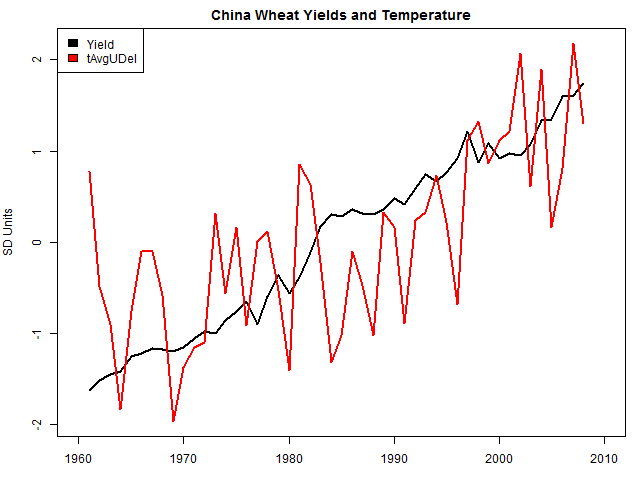
In 2011, I obtained the data for Lobell et al 2011 from lead author Lobell (who undertook at the time to place both data and code online, neither of which appears to be done.) I had asked Lobell to archive code, because it wasn’t entirely clear what he had done. Lobell collated temperature and precipitation data from both UDel and CRU. (For the latter, Lobell used the CRU TS data made famous by the Harry Readme.) In the figure below, I’ve plotted Lobell’s yield and temperature data for the China-wheat combination (both standardised to SD units), as an example of both series going up.

lobell_china_wheat

Lobell regressed Yield (actually log Yield) against time, temperature and precipitation variables, describing the procedure as follows:

Translating these climate trends into potential yield impacts required models of yield response. We used regression analysis of historical data to relate past yield outcomes to weather realizations. All of the resulting models include T and P, their squares, country-specific intercepts to account for spatial variations in crop management and soil quality, and country-specific time trends to account for yield growth due to technology gains (6).

The precipitation and quadratic terms don’t appear to affect the regression very much, i.e. the main effects are delivered by the model in which Yield is regressed against time and temperature as follows:

(1) Yield ~ Year + Temperature

Using conventional regression nomenclature, the regression coefficient b is given by the formula

(2) b= (X^T * X)^{-1} X^T y

where the X matrix of independent variables if {Year; Temperature} and y is the Yield vector.

For convenience (and thus is irrelevant to the point that I’m working towards), normalize the data.

X^T y is simply the vector of correlations of Yield to Time (the normalized trend) and Temperature.

(X^T * X) is nothing more than the correlation matrix between Year and Temperature i.e. the off-diagonal element r is the temperature trend (normalized units) as follows:

| 1 r |
| r 1 |

The calculation of the OLS regression coefficients uses the inverse of this matrix,

| 1 -r | * 1/(1-r^2)
| -r 1 |

The negative term in the off-diagonal means that the OLS coefficient for the regression of Yield onto Time and Temperature is calculated as a function of the correlation between yield and temperature, the trend in yield, the trend in temperature as follows:

b_temperature = 1/(1-r^2) (-r*trend_yield + cor_yield_temp)

In other words, if the correlation between Yield and temperature is less than the product of the trend in yields and trend in temperature (both normalized), then the regression coefficient is negative. This has nothing to do with yields or temperatures, but is a trivial property of the matrix algebra.

As an example, for the Chinese wheat series shown above, although there is a positive correlation between yield and temperature (0.5096), the OLS regression coefficient of a regression of Yield against Year and Temperature results in a negative coefficient. Applying the above formula, the normalized trends (correlations between year and item) for yield and temperature are 0.984 and 0.548, yielding 0.5096- 0.984*0.584 <0.

Gregory et al 2019: Does climate feedback really vary in AOGCM historical simulations?

A guest post by Nic Lewis

Introduction

The recent open-access paper Gregory et al 2019 “How accurately can the climate sensitivity to CO2 be estimated from historical climate change?” discusses, inter alia, the use of regression to estimate historical climate feedback. As I wrote in a previous article, Gregory et al. consider a regression in the form R = α T, where T is the change in global-mean surface temperature with respect to an unperturbed (i.e. preindustrial) equilibrium and R is the radiative response of the climate system to the change in T, however caused; α is thus the applicable climate feedback parameter for that cause. The corresponding effective climate sensitivity (EffCS) is then F2xCO2/α  where F2xCO2 is the effective radiative forcing (ERF) for a doubling of preindustrial atmospheric carbon dioxide concentration. Continue reading

Gregory et al 2019: Unsound claims about bias in climate feedback and climate sensitivity estimation

A guest post by Nic Lewis

The recently published open-access paper “How accurately can the climate sensitivity to CO2 be estimated from historical climate change?” by Gregory et al.[i] makes a number of assertions, many uncontentious but others in my view unjustified, misleading or definitely incorrect. Perhaps most importantly, they say in the Abstract that “The real-world variations mean that historical EffCS [effective climate sensitivity] underestimates CO2 EffCS by 30% when considering the entire historical period.” But they do not indicate that this finding relates only to effective climate sensitivity in GCMs, and then only to when they are driven by one particular observational sea surface temperature dataset.

However, in this article I will focus on one particular statistical issue, where the claim made in the paper can readily be proven wrong without needing to delve into the details of GCM simulations. Continue reading

CG2 and Ex Post Picking

Jul 31, 2019: Noticed this as an unpublished draft from 2014. Not sure why I didn’t publish at the time. Neukom, lead author of PAGES (2019) was coauthor of Gergis’ papers.

One of the longest-standing Climate Audit controversies has been about the bias introduced into reconstructions that use ex post screening/correlation.   In today’s post, I’ll report on a little noticed* Climategate-2 email  in which a member of the paleoclimatology guild (though then junior) reported to other members of the guild that he had carried out simulations to test “the phenomenon that Macintyre has been going on about”, finding that the results from his simulations from white noise “clearly show a ‘hockey-stick’ trend”, a result that he described as “certainly worrying”.  (*: WUWT article here h/t Brandon).

A more senior member of the guild dismissed the results out of hand:  “Controversy about which bull caused mess not relevent.”  Members of the guild have continued to merrily ex post screen to this day without cavil or caveat.

Continue reading

Hack, Now Ex-Bellingcat, Gets Climategate Timezones Backwards

Bellingcat’s Iggy Ostanin, [update: who Eliot Higgins says is now ex-Bellingcat]  recently claimed to have discovered that the nomenclature of Climategate-1 emails was based on Unix timestamps and that the nomenclature proved that Russians hacked CRU from timezone +05:00. Amidst much uninformed hyperventilating. Ostanin’s assertions were swiftly retweeted by Andy Revkin, Roger Harrabin, Ken Rice and many others. However, his claims are backwards – or perhaps, in true Mannian style, upside down.

The connection of CG email nomenclature to Unix timestamps was observed as early as Dec 7, 2009 (see WUWT commenter crosspatch here)m who similarly noticed discrepancies between nomenclature and email times, but concluded that they showed that hacker used a computer set to Eastern North American time (-05:00 Standard).

I pointed the error out on Twitter with technical analysis. I also linked Ostanin to the original WUWT comment making similar point.

Ostanin  responded by claiming that my (correct) replication of CG1 nomenclature was “needlessly complicated” and doubled down with his incorrect assertion that “time seen in hacked email headers is 5 hours behind – to the second – of the time in the decoded email file names”:

Ostanin challenged everyone “to try to see for themselves” – pointing to a internet utility:

After I re-iterated my technical criticism, Iggy stated that he wasn’t “sure if either of [me or Charles Wood] ever came across a Kremlin narrative they didn’t endorse”. Then, in true Mannian (and Eliot Higgins) style, Ostanin blocked me on Twitter.

While it’s a bit absurd to waste time on this trivia, Iggy’s falsehoods remain in circulation. He hasn’t conceded anything. Nor have Revkin, Harrabin, Rice or other re-tweeters conceded that Iggy’s analysis was nonsensical.

In my tweets, I observed that Iggy’s analysis was based on an email sent from GMT timezone and that the 5-hour difference between nomenclature and email time only held for emails from that time zone.  What any competent analyst (and we may safely exclude Iggy from that category) would have done is to compare email timestamp to nomenclature across multiple timezones and Daylight/Standard times. I’ve done so in the table below.

Nomenclature for GMT timezone emails in winter are 5 hours ahead, but only 4 hours ahead in summer. This should have caused Iggy to pause.  Nomenclature for emails sent from Eastern timezone exactly matched the email time – both in Standard (winter) and Daylight (summer) time. Nomenclature for emails sent from Mountain time (two hours behind Eastern) were – 2 hours in both winter and summer.

Ironically, the very first email in the Climategate dossier was sent from Iggy’s Ekaterinaburg (+05:00).  But instead of the nomenclature exactly matching the email time, the nomenclature was 10 hours ahead.

In other words, Ostanin got everything pretty much backwards and upside down. It’s about as bad a bit of analysis as it is possible to imagine. And, instead of simply conceding that he’d made a mistake (which is easy enough to do), Ostanin got belligerent and shut his ears. Unfortunately, Ostanin’s falsehoods are now in circulation and, like Mann’s, will probably fester forever.


PAGES2K (2017): Antarctic Proxies

A common opinion (e,g, Scott Adams) is that the “other proxies”, not just Mann’s stripbark bristlecone tree rings, establish Hockey Stick. In today’s post, I’ll look at PAGES2K Antarctic data – a very important example since Antarctic isotope data (Vostok) is used in the classic diagram used by Al Gore (and many others) to illustrate the link between CO2 and the isotopes used to estimate past temperature. 

Antarctic d18O is one of the few proxies which can be accurately date in both very recent measurements and in Holocene and deep time. However, rather against message, Antarctic d18O over the past two millennia (as for example the PAGES2K 2013 compilation) has mostly gone the “wrong” way, somewhat diluting the IPCC message – to borrow a phrase.

PAGES2017 relaxed the PAGES2K ex ante quality control criteria to include 15 additional series (most of which are not new), but these, if anything, reinforce the earlier message of gradual decline over the past two millennia.

PAGES2K (2017) also added two borehole inversion series, which were given a sort of special exemption from PAGES2K quality control standards on resolution and dating. I suspect that readers already know why these series were given special exemption: one of them has a very pronounced blade.  Long-time readers may vaguely recall that an (unpublished) Antarctic borehole inversion series also played an important role in conclusions of the NAS 2006 report. I tried at the time to get underlying measurement data, but was unsuccessful. A few years ago, when the PAGES2017 borehole inversion series was published, I managed (through an intermediary) to obtain much of the underlying data and even some source code for the borehole inversion. I’ve revisited the topic and I conclude today’s post with a couple of teasers and what is an interesting analysis in works.  Continue reading

PAGES2K: North American Tree Ring Proxies

The PAGES (2017) North American network consists entirely of tree rings. Climate Audit readers will recall the unique role of North American stripbark bristlecone chronologies in Mann et al 1998 and Mann et al 2008 (and in the majority of IPCC multiproxy reconstructions).  In today’s post, I’ll parse the PAGES2K North American tree ring networks in both PAGES (2013) and PAGES (2017) from two aspects:

  • even though PAGES (2013) was held out as the product of superb quality control, more than 80% of the North American tree ring proxies of PAGES (2013) were rejected in 2017, replaced by an almost exactly equal number of tree ring series, the majority of which date back to the early 1990s and which would have been available not just to PAGES (2013), but Mann et al 2008 and even Mann et al 1998;
  • the one constant in these large networks are the stripbark bristlecone/foxtail chronologies criticized at Climate Audit since its inception. All 20(!) stripbark chronologies isolated by Mann’s CENSORED directory re-appear not only in Mann et al (2008), but in PAGES (2013). In effect, the paleoclimate community, in apparent solidarity with Mann, ostentatiously flouted the 2006 NAS Panel recommendation to “avoid” stripbark chronologies in temperature reconstructions. In both PAGES (2013) and PAGES (2017), despite ferocious data mining, just as in Mann et al 1998, there is no Hockey Stick shape without the series in Mann’s CENSORED directory.

PAGES2K references: PAGES (2013) 2013 article and PAGES (2017) url; (Supplementary Information).

Continue reading

PAGES2K (2017) – South America Revisited

The most recent large-scale compilation of proxy records over the past two millennia is PAGES (2017).  They made a concerted effort to archive data (to the credit of Julien Emile-Geay), archiving 692 series, but they perpetuated most other sins within the field.  Rather than abjuring ex post screening, it carried ex post screening to extremes never previously contemplated: tree ring chronologies with negative correlations to temperature are now banished from view altogether. However, its self-professed quality control did not exclude stripbark bristlecone chronologies, which continue to populate the network.

In keeping with my preference to look at regions and proxy types before worrying too much about aggregates, I looked at their South American network, which is an update of the South American network of PAGES2K (2013), which I discussed a few days after publication here.  There were major changes between 2013 and 2017 networks, which were not elucidated in the later study, but which will be discussed in today’s article. The changes illustrate the profound problems with the tree ring chronologies and lake sediment series which make up the vast majority of data in PAGES 2017 and similar studies. Continue reading

A Russian Spearphishing Domain Is Now Hosted in New York City

Central to the Mueller indictment is attribution to Russia of a spearphishing campaign from domains then located in Romania. It is therefore more than a little surprising that one of these spearphishing domains is not only still in operation in May 2018, but hosted in New York City. Continue reading