Update (Jul 28, 2008): On Jan 18, 2008, two days after this article was posted, RSS issued a revised version of their data set. The graphics below are based on RSS versions as of Jan 16, 2008, the date of this article, and, contrary to some allegations on the internet, I did not “erroneously” use an obsolete data set. I used a then current data set, which was later adjusted, slightly reducing the downtick in observations. On Jan 23, 2008, I updated the graphic comparing Hansen projections using the revised RSS version. Today I re-visited this data, posting a further update of this data including the most recent months. While some commentators have criticized this post because the RSS adjustment reduced the downtick slightly, the downtick based on the most recent data as of July 28, 2008 is larger than the RSS adjustment as of Jan 2008.)
In 1988, Hansen made a famous presentation to Congress, including predictions from then current Hansen et al (JGR 1988) online here . This presentation has provoked a small industry of commentary. Lucia has recently re-visited the topic in an interesting post ; Willis discussed it in 2006 on CA here .
Such discussions have a long pedigree. In 1998, it came up in a debate between Hansen and Pat Michaels (here); Hansen purported to rebut Crichton here, NASA employee Gavin Schmidt on his “private time” supported his NASA supervisor, Jim Hansen here , NASA apologist Eli Rabett believed to be NASA contractor Josh Halpern here . Doubtless others.
It seems like every step of the calculation is disputed – which scenario was the “main” scenario? whether Hansen’s projections were a success or a failure? even how to set reference periods for the results. I thought it would be worthwhile collating some of the data, doing chores like actually constructing collated versions of Hansen’s A, B and C forcings so that others can check things – all the little things that are the typical gauntlet in climate science.
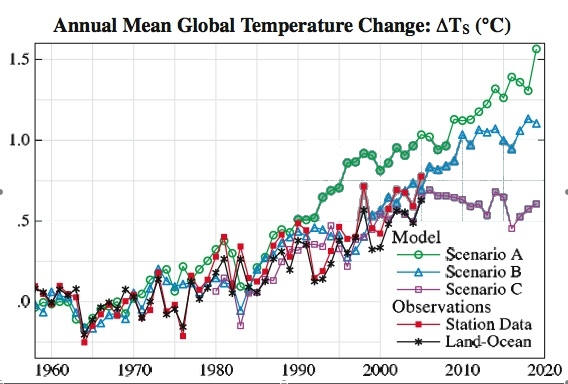
Here is my best interpretation of how Hansen’s 1988 projections compare to recent temperature histories.

I’ll compare this graphic with some other versions. On another occasion, I’ll discuss the forcings in Hansen et al 1988. First, I’m going to review the prior history of this and related images.
Hansen et al 1988
Hansen et al 1988 defined 3 scenarios (A,B, C), illustrated in the two graphics below taken from Figure 3 of the original article. Each scenario described forcing projections for CO2, CH4, N2O, CFC11, CFC12 and the other Montreal Protocol traces gases as a group. In subsequent controversy, there has been some dispute over which scenario was Hansen’s “primary” scenario. In the right panel, only Scenario A is taken through to 2050 and in both panels, Scenario A is plotted as a solid line, which could be taken as according at least graphic precedence to Scenario A. [following sentence revised at Jan 17, 2008 about 9 am] Despite the graphic precedence to Scenario A in the right panel graph, Hansen mentioned in the running text (9345):
Scenario A, since it is exponential must eventually be on the high side of reality in view of finite resource constraints, even though the growth of emissions (`1.5% per year) is less than the rate typical of the past century (~4% per year).
and, then inconsistently with the graphic shown on the right side only showing Scenario A out to 2050, said (p 9345) that Scenario B was “more plausible”, an aside that subsequently assumed considerable significance.
 |
 |
Hansen Debate 1998
In 1998, 10 years after the original article, in testimony to the U.S. Congress and later in the debate with Hansen, Pat Michaels compared observed temperatures to Scenario A, arguing that this contradicted Hansen’s projections, without showing Scenarios B or C.
[Update: Jan 17 6 pm] To clarify, I do not agree that it was appropriate for Michaels not to have illustrated Scenarios B or C, nor did I say that in this post. These scenarios should have been shown, as I’ve done in all my posts here. It was open to Michaels to take Scenario A as his base case provided that he justified this and analysed the differences to other scenarios as I’m doing. Contrary to Tim Lambert’s accusation, I do not “defend” the exclusion of Scenarios B and C from the Michaels’ graphic. This exclusion is yet another example of poor practice in climate science by someone who was then Michael Mann’s colleague at the University of Virginia. Unlike Mann’s withholding of adverse verification results and censored results, Michaels’ failure to show Scenarios B (and even the obviously unrealistic Scenario C) was widely criticized by climate scientists and others, with Klugman even calling it “fraud”. So sometimes climate scientists think that not showing relevant adverse results is a very bad thing. I wonder what the basis is for climate scientists taking exception to Michaels, while failing to criticize Mann, or, in the case of IPCC itself, withholding the deleted Briffa data. [end update]
In any event, in the debate, Hansen responded irately, arguing that Scenario B, not shown by Michaels, was his preferred scenario, that this scenario was more consistent with the forcing history and that the temperature history supported these projections.
Pat [Michaels] has raised many issues, a few of which are valid, many of which are misleading, or half truths, some of which are just plain wrong. I don’t really intend to try to respond to all of those. I hope you caught some of them yourself. For example, he started out showing the results of our scenario A, even though the scenario that I used in my testimony was scenario B…
I don’t have a copy of his testimony and can’t say at this point whether Scenario B was or was not used in the 1988 testimony.
[Update: The testimony is now available and Hansen’s statement that Scenario B was “used” in his 1988 testimony is very misleading: Hansen’s oral testimony called Scenario A the “Business as Usual” scenario and mentioned Scenario B only in maps purportedly showing extraordinary projected warming in the SE USA
On the other hand, Hansen also testified in November 1987 online here and, in that testimony (but not in the 1988 testimony), he did say that Scenario B was the “most plausible”, though in a context that was over a longer run than the 10-20 year periods being discussed here. At present, I do not understand how the trivial differences between Scenario A and B forcings over the 1987-2007 period can account for the difference in reported Scenario A and B results, that’s something I’m looking at – end update]
In any event, Hansen argued in 1998 that real world forcings tracked Scenario B more closely and that warming was even more rapid than Scenario B:
There were three scenarios for greenhouse gases, A, B and C, with B and C being nearly the same until the year 2000, when greenhouse gases stopped increasing in scenario C. Real-world forcings have followed the B and C greenhouse scenario almost exactly. … and the facts show that the world has warmed up more rapidly than scenario B, which was the main one I used.
Here’s the figure from the debate materials:
Hansen and Schmidt
In one of the first realclimate posts (when they were taking a temporary respite from their active Hockey Stick defence of Dec 2004-Feb 2005), NASA employee Gavin Schmidt here tried to defend the 1988 projections of his boss (Hansen) against criticism from Michael Crichton. Hansen issued his own defence here , covering similar ground, citing the realclimate defence by his employee (Schmidt), done in Schmidt’s “spare time”. On the left is the version from realclimate updating the history to 2003 or so; on the right is the image from Hansen’s article, updating the instrumental history to 2005 or so.
 |
 |
NASA employee Schmidt said of his boss’ work (not mentioning in this post that both were NASA employees, although Schmidt’s online profile in the About section says that he is a NASA employee):
The scenario that ended up being closest to the real path of forcings growth was scenario B, with the difference that Mt. Pinatubo erupted in 1991, not 1995. The temperature change for the decade under this scenario was very close to the actual 0.11 C/decade observed (as can be seen in the figure). So given a good estimate of the forcings, the model did a reasonable job.
Hansen re-visited the predictions in Hansen et al (PNAS 2006) – this is his “warmest in a millllll-yun years” article – where he updated the temperature history to 2005, introducing a couple of interesting graphical changes. In this version, the color of Scenario A was changed from red (which is visually the strongest and most attention-grabbing color) to a softer green color. He also plotted two instrumental variants – the Land only and the Land+Ocean histories. Hansen argued that Scenario B was supported by the data and, continuing his feud with Crichton, asserted that his results were not “300% wrong”, footnoting State of Fear. NASA employee Schmidt loyally continued to support his boss on his”spare time” at realclimate, once more visiting the dispute at realclimate in May 2007, re-issued the graphic in substantially the same format as Hansen’s 2006 article, with further changes in coloring. It seems likely that Schmidt, as a NASA employee, had access to the digital version that Hansen used in his 2006 paper and, unlike us at CA, did not have to digitize the graphics in order to get Hansen’s results for the three scenarios. Schmidt stated:
My assessment is that the model results were as consistent with the real world over this period as could possibly be expected
 |
 |
Re-constructing the Graphic
While NASA employee Schmidt, in his “spare time”, has access to NASA digital data, we at CA do not. Willis Eschenbach digitized Hansen scenarios A,B and C to 2005 and I extended this to 2010. The three scenarios to 2010 are online here in ASCII format: http://data.climateaudit.org/data/hansen/hansen_1988.projections.dat
In the graphic shown above, I’ve compared the NASA scenarios to two temperature reconstructions: the NASA global series and the RSS satellite series (not showing CRU and UAH versions to reduce the clutter in the graphic a little.) The GISS temperature history has been used in the prior graphics and the RSS version has been preferred by IPCC and the US CCSP.
In order to plot the series, several centering decisions have had to be made. The GISS GLB (and other series) is centered on 1951-80, while the three scenarios were centered on the control run mean. The 1951-1980 means of the three scenarios, which included forcings for the period, were thus higher than the 1951-80 zero for the target temperature series by 0.1 deg C for Scenario A and 0.07 deg C for Scenarios B and C. The scenarios were only available in digital form for 1958-1980. For the GISS GLB series, there was negligible (less than 0.01 deg C) difference between the means for 1958-1980; 1958-1967 and 1951-1980.
In order to put the three Scenarios apples and apples to the GISS GLB temperature series (basis 1951-1980), I re-centered the three scenarios slightly so that they were also zero over 1958-1967. This lowered the projections very slightly relative to the instrumental temperatures. (Lucia recognized the problem as well and dealt with it a little differently). I applied a similar strategy with respect to the satellite series which did not commence until 1979. In this case, I re-centered it so that its 1979-1988 zero matched the 1979-1988 values of the GISS GLB series. This yielded the diagram shown above:
Comments
I’ll talk some more about the forcings in a day or two.
I’ve shown 1987, the last year of data for Hansen et al 1988. The 2007 RSS satellite temperature was 0.04 deg C higher than the 1987 RSS temperature and there was substantial divergence between Scenario B in 2007 and the RSS satellite temperature (and even the GISS temperature surface temperature series). Strong increases in the GISS Scenarios start to bite in the next few years. To keep pace, one must really start to see increases in the RSS troposphere temperatures of about 0.5 deg C. sustained over the next few years.
The separation between observations and Scenario C is quite intriguing: Scenario C supposes that CO2 are stabilized at 368 ppm in 2000 – a level already surpassed. So Scenario C should presumably be below observed temperatures, but this is obviously not the case.
It should be noted that Hansen et al 1988 considers other GHGs (CH4, N2O, CFC11 and CFC12). Methane is a curious situation as methane concentrations may have stabilized – making the SRES methane projections in even the A1B case possibly very problematic.
References:
Click to access hansen_re-crichton.pdf
http://rabett.blogspot.com/2006/04/rtfr-i-rather-strange-push-back-has.html
Click to access 1988_Hansen_etal.pdf
http://sciencepolicy.colorado.edu/prometheus/archives/climate_change/000771out_on_a_limb_with_a.html
rankexploits.com/musings/2008/temperature-anomaly-compared-to-hansen-a-b-c-giss-seems-to-overpredict-warming/
Click to access SPFtranscript.pdf
rankexploits.com/musings/2008/temperature-anomaly-compared-to-hansen-a-b-c-giss-seems-to-overpredict-warming/
http://rankexploits.com/musings/2008/how-gavins-weather-vs-climate-graphs-compare-to-hansen-predictions/
http://sciencepolicy.colorado.edu/prometheus/archives/climate_change/001318real_climates_two_v.html
http://illconsidered.blogspot.com/2006/04/hansen-has-been-wrong-before.html
http://www.climateaudit.org/?p=796


201 Comments
Here’s a script to generatre the above graphic. The script is online in ASCII form at http://data.climateaudit.org/scripts/hansen/hansen_1988.projections.txt if you have trouble converting Unicode signs here.
Hmm, curious. I suspect Hansen was feeling good about himself in 1998. His scenario B (and C to some extent) appered to track and trend well with his predictions, but the following years, 1999 and 2000, likely gave him a few sleepless nights. Todays comparison to observed is off the mark and heading in the wrong direction, which is where many will likely take the conversation.
However … despite my feelings toward the man, one must acknowledge his abilities to model (guess) climate well for approximately 15 years. I wish I could do the same for my retirement portfolio.
I had a related thought. It’s easy to “feel good about” one’s forecasts if one cherry picks time frames so that observed slopes are as steeply alarmist as one’s predicted slopes. As Steve M writes above, Hansen et al (1988) was published following a major El Nino. Meanwhile MBH98 was published following a monster El Nino. Based on the decadal pattern here (granted, n=2 cycles!) we can predict that the next major El Nino should result in another landmark publication where the hypothesis of an alarmist trend is resurrected. Shall we say … 2010? At that point GHG scenario C may start to look plausible again.
Thanks to Steve M and lucia and Willis for working up these graphics in the form of turnkey scripts.
Daniel Klein asked a few weeks back of Gavin Schmidt what it would take to falsify AGW. I think that dialogue is now relevant here. (If not, Steve M, feel free to delete.)
#529 of unthreaded #28
#549 of unthreaded #28
[I note that Daniel Klein has learned to genuflect after asking any critical question.]
And finally #553 from unthreaded #28:
It would be nice if we could keep this thread at a high level of civility and analytical correctness, and eventually get Gavin Schmidt to comment. I would really like some clarity as to how the ensemble of model runs are whittled down into a narrower subset without comprimising the ability of the model to “span the full range” of “weather noise”. What are the REAL confidence intervals on those ensemble runs? You need to know that before you start comparing observed and predicted time-series.
The nested blockquotes that I used in #4 did not work at all and now that comment is a disaster.
Is it possible to fix this? Nest blockquotes used to work.
Steve: IT doesn’t seem to anymore. I suggest italicizing the second nest of quotes. I tidied the above post for you.
In Gavin’s first plot he had just used the obs to 1998 which showed them falling between scenarios A and B. Then someone asked him (in the RC comments) to add the post 1998 data. He did so and, as you can see above, the obs then appeared to follow scenario C. A very short time after this there was a (coincidental?) publicized adjustment to the GISS data and you can see the effect on Hansen’s subsequent graph – the obs from 1992 onwards have been shifted up and they follow scenario B again. Shortly afterwards, Hadley then also made adjustments which brought their own graph back into line with GISS.
Yet he carried over the shaded area of the altithermal/eemian temps (listed as 6000 and 120,000 years ago, respectively). This flies in the face of the “warmest in a millllll-yun years” idea.
Using that shaded area seems to say that we are at least as warm (but not warmer than) as we were 6000 years ago.
And I’d still like to see which article he used as a reference to that idea.
#4 Bender
Many thanks for reprinting this very interesting and revealing interchange from RC, which I totally missed. I think Daniel Klein asked a really good question and in effect got Gavin to provide some confidence intervals around the projections. If I understand correctly that the models will have to be significantly rethought if the 1998 global temperature record is not exceeded by 2013, assuming no exogenous negative forcings. In adding an additional 5 years, I think Gavin is being a bit cute here and that the first statement indicating a decade is more reasonable – a math wiz here can probably come up with the difference in probabililites the additional 5 years makes. But more to the point, the decade estimate would mean that we would expect some significant reassessment of the models after THIS YEAR, 2008!! – prior to the next el Nino. (Your point in #3!) Is
Gavin playing poker or doing science?
Hansen’s testimony should be available in the Congressional Record of the 100th Congress. Unfortunately the online version at Thomas starts with the 101st Congress, and the online version at the GPO starts with the 104th Congress. The index though is searchable and has two listings, D429 23JN and D469 7JY. There is a document for a hearing on global warming before a House subcommittee on Energy and Power that took place July 7 and September 22 1988. Its SuDoc Number is Y 4.En 2/3:100-229 and its item number is 1019-A or 1019-B (microfiche). My GPO search showed there were three other hearings that year that mentioned global warming in the hearing title, none that were on the 23rd of June.
If anyone has easy access they could find these, some have been distributed to local libraries. Or obtain it through the GPO.
http://thomas.loc.gov/home/thomas.html
http://catalog.gpo.gov/F
Because we cannot tell what the real starting point for the projections/observations is …
… (is it 1958?, the 1958 to 1967 mean, 1984 (the last year of observation data Hansen says he used), 1987 (the last year of observation data Hansen would have had in 1988) etc. etc.) …
… this graph is susceptible to manipulation and whenever Gavin or Hansen or RealClimate plot it, they can make it look like the projections are very close to bang on.
As well, greenhouse gas emissions turned out to be between Scenario A and Scenario B (CO2 is closer to B but Methane is closer to C), so that also gives them some wiggle room.
I prefer using 1987 as the starting point. The 1987 RSS anomaly is +0.13C and the 2007 RSS anomaly is +0.16C. Twenty years later and lower atmosphere temperatures are only 0.03C higher.
I will send by email attachment the Hansen 062388 senate testimony transcript, written oral and attachments.
Steve: Received -thanks very much. These are now online here http://data.climateaudit.org/pdf/others/Hansen.0623-1988.oral.pdf and http://data.climateaudit.org/pdf/others/Hansen.0623-1988.written.pdf
He’s poking science.
I’m not sure why a volcanic eruption would automatically constitute a global cooling. I know a lot of ash and particulates (aerosols) are thrown up, but volcanoes also spew tremendous amounts of CO2, don’t they? If CO2 is so powerful why doesn’t the CO2 forcing override the aerosol effect? Maybe because CO2 forcing is logarithmic after all, and has very little effect at this point.
When say the Social Security Administration gives three projections of the system’s condition, ordinarily these are best case, worst case, and most likely case. So I think it’s reasonable to take Hansen at his word that case B was his most likely estimate, and not to read too much into his color choice.
Personally, I usually start with darkish blue since it looks nice in color and prints well in B&W. Then red, since it contrasts well with blue in color, and is a little lighter in B&W. Then green since it comes out a little paler than red in B&W. If I wanted to emphasize a line, I would try to make it the blue one, not the red one.
Steve: In mineral promotions, red is nearly always used to highlight the spot of interest.
Looks like maybe model variables were tweeked to create a best fit with observations. That yeilded pretty good results for a while, but when the trend that was occuring at the time the original model scenarios were run began to change, his results diverged from reality. GCMs have limitations and whole system is not understood enough to accurately model IMHO.
Re Glacierman in post 14
Perhaps what we see now is a climatological application of Goodhart’s Law?
Steve- Thanks for posting this. Here are some references that may be of some use for looking at the individual forcings in the scenarios:
Hansen, J., and M. Sato 2004. Greenhouse gas growth rates. Proc. Natl. Acad. Sci. 101, 16109-16114, doi:10.1073/pnas.0406982101.
http://www.pnas.org/cgi/content/full/101/46/16109
Most recent data on forcings:
http://www.esrl.noaa.gov/gmd/aggi/
Glacierman,
I think you are correct, bender said as much in #3. That said I doubt anyone has modelled the variability of the stock market as closely as Hansen has modelled the variability of Earth’s climate. Perhaps Ross could say a word or two about that.
I am not a fan of Hansen, he has many apologists, but strip away his bluster and political activism, you have a very smart individual and respected (in some circles) scientist. If he were not deviously clever, we would not be talking about him.
In many ways, Hansen (the so-called Shepherd of AGW) reminds me of Stephen Jay Gould (the controversial palaeontologist). Gould was to evolutionary psychology, as Hansen is to GW scepticism. He would infuriate his critics with his essays, books, and pet theories, but after he passed, his critics longed for his sharp mind.
RE #13,
Here I thought gold was their preferred color! ;=)
Another posting by NASA employee Gavin Schmidt defending Hansen, not mentioned in the above, was on December 2, 2004 here http://www.realclimate.org/index.php/archives/2004/12/michaels-misquotes-hansen-again/ , which appears to be Gavin’s very first post at realclimate (Dec 1, 2004 is the date of the realclimate introduction post.)
Gavin posted his defense of his boss in his “spare time”, which in this case occurred in the middle of a 9 to 5 Thursday. I wonder if Gavin booked Dec 2, 2004 off for “personal business”.
If you browse http://www.realclimate.org/index.php/archives/2004/12/ you’ll see how much effort they were then putting into preemptive strikes defending the HS ( MM2005 was then about to be published) and you’ll see why John A convinced me that I needed to try to defend myself. Thus, CA was born a couple of months later in Feb 2005 (carrying over a few website comments).
#13 In nature red is the universal color of alarm. Some smart googler could probably find a Nature paper on the topic.
Steve:
I believe these are the actual links
http://data.climateaudit.org/pdf/others/Hansen.0623-1988%20oral.pdf
http://data.climateaudit.org/pdf/others/Hansen.0623-1988%20written.pdf
I think there was a typo.
Comments on Hansen 062388 Testimony
Hansen bluntly says to the Senate that Scenario A is “Business as Usual”. In the first part of the talk, he talks about global climate. Then goes on to talk about summer heat spells. (This may have been a hasty concoction, as on that day in the summer of 1988 it was extremely and unusually hot in Washington DC. )
The written documents submitted with the oral talk follow one another closely as to content. A preprint of Hansen et al 1988 is included, along with the three viewgraphs that were presented.
As far as the “summer heat wave” section of the talk, Hansen discusses maps – not graphs – which have as the underlying basis, Scenario B. This is where all of the vague beliefs about “Hansen only talked about Scenario B” originate from.
Ten years later, when Michaels gave his Congressional presentation, he was addressing the primary prediction made by Hansen in 1988. That of course nothing to do with the sensational “summer heat waves” talk of ten years prior. There is of course no discussion of maps.
Rather it was on the primary topic – global warming. Michaels was dead on correct to note that Hansen’s prediction of 0.4C temperature increase was wildly incorrect.
Hansen’s phrase to the Senate was exactly as Michaels clear stated, “Scenario A was business as usual”.
The smearing of Dr. Pat Michaels was completely unjustified. Michaels presented the relevant prediction, Scenario A, “business as usual” in 1998.
#21 Interesting. He thought he could fool the politicians by cherry-picking his endpoint, 1987-88 – a choice, due to El Nino, that grossly exaggerates his trend. (Look what happened in 1989: La Nina.) He is smart enough to know what he was doing, in terms of creating a statistical distortion. He was sounding the alarm, promoting an activist agenda. And does anyone see any mention of a “precautionary principle”? All I see are distorted facts.
In 1988, Scenario A is the status quo scenario – Hansen’s “business as usual”. Therefore, the plain language interpretation is that assuming that nothing changes this is what Hansen’s models predict. The charts show that actual observations, whatever their flaws, immediately began to deviate from this scenario. This seems to be a case for rethinking the models and explaining how and why the physical assumptions underlying the model
need to change.
Moreover, since observations now appear to track Scenario C – a drastic reduction in GHG – and there appears to have been no such reduction, then again the assumptions underlying the model need to be made explicit and re-assessed.
Is it all this simple?
Finally, a lot seems to depend on treating 1998 as part of a trend rather than an aberration. If that one year was dropped or replaced with a 5 year mean, what would it do to the trends. This is another version of when will 1998 be surpassed. If it is not surpassed in the near future then it loooks more like an anomaly.
#15
Def. of Goodharts Law: `When a measure becomes a target, it ceases to be a good measure.’
I agree with Ian #17, he is a very smart guy. Smart enough to know how to make a trend seem as dire as possible by picking dates. If he is right, then placing activism and alarmism above scientific principals will make him a hero. But I believe that his actions are actually fueling the counter case to what he has been advocating. If he/they are so accurate and correct, their work should stand up to any scrutiny.
Thanks Mhaze.
I do not see any mention of a “preferred” outcome. Nor is there a “worst case”, “expected”, “best case” organization in either oral or written testimony. Instead, A is presented as business as usual, what would happen if the trace gasses continue growing at an exponential rate, B is some sort of reduced linear growth and C is drastic curtailment of emissions with everything cut off by 2000.
A is clearly our not doing anything. Going back 10 years later and saying B fits the data is different than highlighting what happends if we don’t do anything. If he wants another re edit, he could claim he saved us from A. Isn’t he arguing now that the reason that we are seeing C is that the MDOs are covering up the growth?
Steve
Did you hear Gavin Schmidt’s statements on the acceleration of global warming, tipping points etc on PBS Radio yesterday morning? PBS had him on for a whole hour
http://wamu.org/programs/dr/08/01/16.php#18143
I’ve been browsing some of the controversy over Hansen’s projections. NASA employee Gavin Schmidt said:
As noted above, in his debate with Pat Michaels, Hansen stated:
I agree entirely with Mhaze characterization of Hansen’s 1988 testimony, now available online at CA. Hansen said in his testimony:
Scenario B is only mentioned in the following context in the oral presentation:
This regional prediction is worth re-visiting in itself – it seems to me that our USHCN discussions have shown that USHCN temperatures have increased more in the west than the southeast (where, as I recall, there has been cooling.)
Hansen said in 1998:
Yes, he used Scenario B to illustrate regional effects, but there is no indication in his testimony that he regarded Scenario B as the “most plausible”. But the transcript shows that he identified the “business-as-usual” case as Scenario A.
I wonder how NASA employee Gavin Schmidt, in his “spare time” of course, would characterize Hansen’s 1998 statement on a scale ranging from “simple confusion” to “pure dishonesty”.
sorry for the digression, but is not the difference in Hansen’s scenarios mearly the model boundary conditions (primarily, the change in ambient GHG concs over time?). Asside from the arguments over who is being dishonest about the testimony…didn’t scenario B turn out to be closer to what actually happened RE said boundary conditions and so should not that be the proper comparison result (over time) for the Hansen model at this time?
Thanks
So it seems to me we have a total error of Actual-Scenario A.
However, we can decompose that to:
Model error = Actual-Scenario B
Assumption error = Scenario B-Scenario A
And even this would be based on an assumption that the three scenarios were entirely exogenous factors.
This is such a telling observation
From the written testimony, page 48, description of figure 3:
This is quite revealing of the Hansen point of view at the time of his testimony.
I’m willing to bet that the growth in CO2 since 1988 has been much closer to the “business as usual” run, than it was to any of the other runs.
Hansen writes on p. 9345 of his 1988 paper:
“Scenario B is perhaps the most plausible of the three cases.”
Click to access 1988_Hansen_etal.pdf
He explains what he means by this:
“Scenario A, since it is exponential, must eventually be on the high side of reality in view of finite resource constraints and environmental concerns . . .”
He also says on p. 9343:
“Scenario A assumes that growth rates of trace gas emissions typical of the 1970s and 1980s continues indefinitely . . .”
Thus, I think it is appropriate to conclude that over the period to 2007, Scenario A is equivalent to what the IPCC calls its “no policy” scenarios, which mean business as usual without explicit policies implemented to limit emissions. When Hansen said “most plausible” he was factoring in factors such as limitations on fossil fuels and eventual emissions policies, which may certainly be the case over the longer term but have not interrupted BAU as yet.
The accuracy of his scenarios to replicate what actually happened since 1988 is another question (stay tuned, more on that shortly).
As an aside, I note that in section 5.2.4 of the paper Hansen compares 7 years of observational data with the model runs. Gavin Schmidt went nuts when I compared 8 years of data with a model prediction (and I even concluded that little could be said on that time scale).
The more general conclusion is that forecast verification make climate modelers very nervous. It shouldn’t. Weather forecasters bust forecasts all the time and learn from it without going nuts. of course, weather forecasters have never been so bold as to claim that all of their forecasts are always right.
#25 bender: “Hypothesis: GHG/AGW may be happening, but the effect is far weaker than what these partisan pseudoscientists claim.”
This is exactly the point. AGW may be happening, but so far the effect has been entirely indiscernable. 20th century climate wanderings have been historically unremarkable and indistinguishable from normal happenstance.
35 MarkW says:
It depends on what he meant by “about 1.5% yr-1 emission growth”. If he was talking about the CO2 output by humans then Scenario A matches reality. If he is talking about the CO2 concentration in the atomosphere then he can argue that the acutual CO2 growth was less than what was assumed by Scenario A.
#37 RPJ
Not another AGW double-standard? From a modeler no less! Shameful.
Just noting that trace gases (CFCs and Methane) did meet the case of Scenario C. CFC concentrations have fallen now and Methane levels have stablized.
It is not really clear, however, what Hansen was assuming for CO2 in his Scenarios (CO2 and N2O have continued increasing at the trends of the mid-1980s.)
Concentrations of the GHGs from 1979 to 2006 are shown in the chart at this link.
Re 13, Hu, Steve
In the CS world, red (or red-orange) is almost invariably used for the warmest temps, AL on maps. So that may explain the orig color choice.
Cheers — Pete Tillman
I just received my monthly issue of one of the trade mags I get. It has a “lessons learned” article in it about Challenger. I will read it with great interest. There is what I consider to be an out of control management system at NASA. I will report out on the article later.
bender says, It would be nice if we could keep this thread at a high level of civility. Umm, too late McI’s original post crossed the civility line. I keep reading deniers claiming this site is scientific but it appears to be more catty than the girls lockeroom in a high school.
The Hansen et al 2006 paper makes some interesting statements:
It’s unusual not just because of its magnitude, but because the GCMs don’t predict it. The GCMs are underestimating internal climate variability, which despite its “regionality” nevertheless contributes massively to globally averaged statistics.
Proving that Hansen is fully aware how statistical distortions may arise from cherry-picking 1988 or 1998 as convenient dates to publish “landmark” papers.
“Say it three times every night before going to sleep*”: when the solar cycle peak coincides with El Nino it is time to sound the alarm.
* -raypierre
Here is a graph showing Hansen’s CO2 component of the relevant scenarios vs. observations 1984-2006.
The difference between A and B is irrelevant on this time scale, and both perform better than C (obviously). You can see Hansen’s version of this (without the obs) in the top of Figure 2 in his 1988 paper.
#44 Winnebago
Just so we’re clear, there is nothing civil about the term “denier”.
Scenario B is perhaps the most plausible of the three cases.
what exactly is the reason for further debate?
Meanwhile, in la-la land, gavin Says:
11 January 2008 at 2:14 PM
http://www.realclimate.org/index.php/archives/2008/01/uncertainty-noise-and-the-art-of-model-data-comparison/langswitch_lang/sw
This is special pleading, and it is fatal to Schmidt’s entire argument that the predicted and observed trends match. Maybe someone can pre-empt me and explain why? [Hint: I will simply invoke the only argument available to him when he was desperately trying to rebut Douglas et al.: the error on the GCMs is enormous.]
More later on the GS/RC double-standard on “weather vs climate” and “internal vs external variability”.
Pat Frank said (January 17th, 2008 at 11:40 am
This is exactly the point. AGW may be happening, but so far the effect has been entirely indiscernable. 20th century climate wanderings have been historically unremarkable and indistinguishable from normal happenstance.
If you really want to see how “unremarkable” they’ve been, put an upper line (through the grey area) corresponding to the 39-40 high temp.
The temperature trends for the US regions can be generated here . I see no alarming temperature trend in the southeast or midwest for the time period mentioned by Hansen. A regional precipitation plot is harder to generate but I think it will show nothing abnormal also.
On global temperature trends, one thing to note is that the 1997-2001 period was one of a strong La Nina (cool) followed by a strong El Nino (warm) followed by a strong La Nina (cool). This pattern masked (my conjecture) a “background” rise in global temperatures over that period, instead making it look like there was a rise circa 2000-2001 rather than 1995-2001.
My belief is that much of the 1995-2001 “global” rise was related to warming of the far north Atlantic (see here for the warm-season SST pattern). This warming released both sensible heat and humidity into the Arctic region, resulting in this Arctic/Subarctic air temperature increase .
If this far north Atlantic SST rise is related to the AMO and has peaked, and if the PDO is switching back to a cool phase which reinforces La Nina activity, then the global temperature pattern may be sideways for quite a few years. That would be a problem for gavin and Hansen.
It seems ro me that in order to assess the accuracy of the models, you first need to check their assumptions. For instance, I think someone mentioned a scenario which had several volcanic eruptions between 1988 and now. But did these actually happen? And which scenario’s CO2 is closest to actual? I know Roger posted something above, but it seems to me that the only apples to apples comparison you can do is to rerun the models with what actually happened (the actual volcanoes, El Ninos, La Ninas, and emmissions.) But for that you’d need the code for the models. I’m not clear, but is that public? Can you get it?
On which scenario was primary:
I think you should take Hansen at his word that he always thought scenario B was the main one at least in some sense. I can’t find any spot in the paper where he calls this out, but when he showed detailed geographical predictions, he used scenario B.
Why was scenario A run longest? I have no idea. You’d have to ask Hansen. However, I can suggest a reason that is consistent with A not being the main computation. First, scenario A was run longest because it was run first. (See page 9342 just before section 2.)
So, why was scenario A run firsts? Well, NASA scientists do have bosses and program managers. I will also speculate that the forcing for scenario A was selected partly to foster discussions with programmatic types and to convince program managers that study was required. It actually fairly routine to do bounding calculations to show whether or not further review should be done, and “A” has the fingerprints of that sort of thing.
Had A shown nothing, B & C would never have been run. B&C were only run because A was not the main scenario.
On access to raw data:
I disagree with some of the choices Gavin made when comparing the Hansen’s model to data, and I disagree with his conclusions.
Still, I think this is unfair:
When I asked Gavin for the scenario temperature anomaly data in a comment at RC posted during Christmas break, he provided that data (I think about a week later). He also proactively provided files for the forcing data, which I hadn’t requested.
Gavin says the ABC anomaly data were digitized from the graph, but evidently not by him. My plots at my blog use those data. Gavin isn’t an author on the 1988 paper and I suspect he didn’t have access to the raw data.
I’d go furter and speculate that NASA’s programmatic requirements didn’t require Hansen to keep a file of the data points and the raw data no longer exist. ( I could grouse about gov’t agencies here. But, this is not, strictly speaking the fault of the individual scientists who may not remember to back up 1988 data and subsequently store it on easy to retrieve media over the course of two decades, which may involve moving to different offices, buildings etc. At Hanford, with waste tank work, we had specific requirements for keeping data imposed by program managers. The rules were a pain in the *&%, but they ensure that, eventually, key information can be obtained should things go wrong later. )
On resetting the baseline:
I don’t think there is an officially good way to reset the baselines given data now available and published. I wish modelers were in the habit of reporting the real honest to goodness thermometer temperature corresponding to the baseline. If they did, we’d at least have a preferred pin point.
I read a blogger somewhere suggest they just stick with Hansen’s first choice. That’s fair in some sense. But, on the other hand, he was able to eyeball agreement between 1958-1983 before publishing. Since the zero point for the baseline is rather arbitrary, it might be difficult for him to be entirely objective and avoid selecting one that showed the best agreement.
Right now, figuring out just how close the models and data are is a bit of a cherry pickers dream. Shifting the baseline within reasonable bounds alters one’s conclusion. Shifting the measurements around also do.
The one thing that is true: The models predict up. Temperatures went up. So, the values are qualitatively correct. Unfortunately, that still leaves a very wide uncertainty when using these to extrapolate forward.
@John Lang–
On the dividing point for projections/ predictions. It’s best not to pick the starting point for comparison based on the the temperature measurements themselves, or the results you want to get. This is already sort of a cherry pickers dream, but still, there are some rules making some cherries off limits!
I recommend looking at dates associated with when the work was initiated and first made public.
The manuscript was submitted in Jan 25, 1988. Given clearance processses at most labs, I think we can be confident the manuscript was, for all intents and purposes, complete no later than Thanksgiving 1987. Still, it’s unlikely the scientist finished computations in 1986 and left the data in a box for a year waiting to see if their prediction for 1987 was right. So, 1988 is the plausible date to beging testing forcast ability; 1987 is not.
The paper itself says computations for transients began in 1983, and results for scenario A were presented at a meeting in 1984. So, 1984 is the earliest possible data for testing forecast ability. At that point, the model was frozen, and other scenarios were run. Earlier results are, strictly speaking “post dictions”.
I picked 1984 to test the model. But, I think if you are trying to be fair, you need to pick 1984 or 1988. Picking 1987 is really sifting those cherries.
The dialogue on this topic at RC is absurd, reduced to a strawman yes/no AGW by the consistent, concerted efforts of gatekeepers Hank Roberts and Ray Ladbury, among others.
The opening post by GS is convincing to me that it is unlikely that a positive, err, “trend” in temperature has abated since 1998. My question concerns the quantititative estimate of the slope of that trend. The gatekeepers’ job is to steer discussion toward yes/no debate on AGW, and away from a scientific discussion of the magnitude of slopes on those 8-year trend lines and the contribution attributable to CO2. The uncertainty on the slopes is high, and the proportion that can be attributed to CO2 even more uncertain. They do not want you to talk about that. They want to push the skeptic back to the less defensible, categorical position that GHG/AGW=0. Much easier to win that argument.
You nailed it exactly right David. This is exactly the theory that I have espoused, and you are the first person I have seen to echo it so succinctly. Thanks for putting in writing here what I never rose to the occasion to do.
I have a question. Where do the “wiggles” in the 1988 projections come from?
This was not immediately evident from skimming the original Hansen paper. If the model is deterministic, one would expect that the result would be smooth whether the solution oscillated or not. It can’t come from other variables expect as boundary conditions since the future behavior of those other variables would not be known. I did notice from Figure 2 in the paper that they threw in some hypothetical volcanoes for the years 1995, 2015 and 2025 presumably to create an aura of “reality” for their model. Did they also create hypothetical variations for the other factors? I presume that there were no randomly simulated components in the model because a result based on a single run of such a model would basically be meaningless with no indication of how the randomness affects the results. The wiggles make the projections look like a “real” temperature series, but how did they get there?
In Hansen’s discussion with Michaels, he states the model scenario contained a large volcano. It turns out there was a volcano in the projected time period and Hansen claims models B and C followed actual measurements.
If a volcano is modeled, why isn’t an El Nino also modeled which would tend to increase the projected temperature changes?
re 52. hadley and hansen are already handicapping 2008 as cool
That you can approximate a 30-year ‘trend’ using a sequence of shorter trend lines (e.g. 8 years) does not imply the 30-year pattern is a GHG-caused trend. LTP/ocean upwelling can generate low-frequency anomalies that look like increasing trends over very short (relative to ocean circulation) time scales. Same for decreasing (or abating) “trends” – a point that agrees with DS’s #52.
lucia says
Therein lies the problem.
Depending on when he’s speaking, which scenario is primary has changed.
There are no wiggles in the ensemble error bars – which I have only ever seen plotted once – when GS was trying deperately to refute Douglas & Christy.
@bender–
Yes. For many people seen as deniers/ skeptics, the question is not “yes/no” it’s “how big”. There is a huge difference between Scenario A and Scenario C. A definitely over estimates. Scenario C may over estimate, but not so badly that we can say it’s wrong with any high degree of certainty.
That said: I doubt the warming trend has ended. I just doubt it.
ENSO is an ’emergent property’ of the ocean circulation. Therefore it *is* modeled, in the sense that all the thermodynamic and fluid dynamic processes that are thought to produce these kinds of effects are included in the GCMs. The only problem is that these features don’t emerge the way they are supposed to.
So do I. But human intuition is fallible. So we measure and we model and we try to be objective about how the models are performing.
lucia, would you have predicted the flattening of global CH4 in 1999?
Bender– I don’t predict forcings. 🙂
I just predict temperature given a forcing history. My current post-dictions are a little high, but slightly better than Scenario C.
I came up with the idea for my model on Sunday night (I think.. maybe Saturday.) The first cut gives me a correlation coefficient of 0.89 (as Excel calculates it. I have issues with that for this particular model. I’ll be calculating a real one later– I think I’ll look worse. But it’s still pretty good.)
Once I get this nailed down, I’ll be able to run all sorts of “thought experiments” quickly. Of course, the thought experiments will only be meaningful to those who think my model describes anything realistic. 🙂
lucia says:
Humans used to looking at various economic graphs which tend to always go up in the long run (population, stock market, housing prices, etc). I think this gives most humans a bias toward expecting continuous upward trends with periods of dips. Natural processes are different and do not follow the same rules. A phase reversal on the PDO or another Dalton minimum could send temps falling again no matter what the science of CO2 says.
In reality Scenarios A, B or C as proposed in 1988 hardly matters 20 years later – it is whether actual observations support the underlying assumptions of today’s models and at what point do the model builders acknowledge and explain how they have adjusted the models to fit with new observational data. (How Hansen et al dealt with the more contemporaneous discussion of these Scenarios, is another matter.) That is why I think Daniel Klein’s question and Gavin’s response is so interesting. If Gavin et al are seeing 2008 as a cool year, we should expect some serious reconsiderations of the assumptions underlying the model – but then Gavin punted to 2013 and we have to wait. If we stick with 2008, it brings us neatly back to Steve’s question of where the 2.5C for doubling of CO2 comes from – since this is surely the crucial assumption underlying these models.
– Conventional wisdom, 2006.
Bender (comment #4), I brought up on RC one confounding effect that probably needs to be considered with respect to anthropogenic global warming.
If we take seriously the flattening out of the global mean temperature (i’m not suggesting that we should), this might be explained by a simultaneous improvement in CO2 emissions by industrialized nations coupled with increased aerosol production in third world nations. I know some people (e.g., Singer) are nervous about the link between CO2, aerosols and global temperature. Indeed they tend to regard the introduction of the aerosols as a “hack” to explain away the lack of warming in the 1945-75 period.
I write it off as a very real effect that is not well characterized by the models, probably because these models don’t model with enough accuracy the effect of the additional aerosol particles on cloud production to properly account for it’s full effect on temperature.
In any case, if I’m correct, then the apparent failure of Hansen’s prediction was not to foresee the industrialization of the 3rd world nations and its ramifications, and not some more basic problem with his climate model.
Bernie says:
What you are describing is a catch 22 situation. We can’t evaluate the new models because there is not enough data. But we can’t evaluate the old models because they are out of date. We can’t do much about the lack of data but we can evaluate the old models.
RE: #68 – Mother nature loves oscillations, and superpositions of many different oscillations at different frequencies. Meanwhile the Naked Ape, has more of a linear perception bias hard wired into its brain. Some of the longer lived civilizations have learned to somewhat overcome it with a more cyclical philosophical perspective, but here in the West, this hard wired bias rules supreme.
Sorry I meant #66 … AKA “Raven says: January 17th, 2008 at 2:11 pm”
That is a dodge, but your smiley gets you off the hook. 🙂
To a climatologist CH4 may be a forcing, but to a biogeochemist it is a response. So let me rephrase. Would the amateur biogeochemist in you have predicted a flattening of CH4 in 1999? The amateur economist a housing market collapse in 2007? And so on. Things happen in dynamic systems.
Steve,
I took your method of zeroing the three projection scenarios:
and re-zeroed the GISS surface-ocean data to the same 1958-1967 period. Here is my scorecard for the 20 years (1988-2007) of out-of-sample projections:
Hansen A:
Average projected anomaly: 0.82 C
Average actual anomaly: 0.39 C (48% of projected)
20 of 20 years projected anomaly exceeded actual anomaly.
Hansen B:
Average projected anomaly: 0.58 C
Average actual anomaly: 0.39 C (68% of projected)
18 of 20 years projected anomaly exceeded actual anomaly (all but 1997 and 1998)
Last projected anomaly less than actual: 1998
Hansen C:
Average projected anomaly: 0.49 C
Average actual anomaly: 0.39 C (80% of projected)
17 of 20 years projected anomaly exceeded actual anomaly (all but 1988, 1996, and 1998)
I’d say scenario A is not only dead, it’s long dead.
As mentioned above, the forcing assumptions of scenario C have proven to be way off, so that one is pretty well dead, too.
Which leaves scenario B hanging on life support at best, with the last sign of brain-wave activity being the El Nino year of 1998.
@Raven–
I rarely look at econometric data. I’m a mechanical engineer. I tend to think of the world in terms of mechanics and thermo-dynamics. I’m used to the idea things go down– gravity tend to pull things in that direction. 🙂
But yes, phase reverals on the PDO could do dramatic things, and I understand that lowering temperature could be one of them.
@bender-
There is no amateur bio-geochemist inside me. Or, if such a thing lurks within, it’s a very stupid ill-informed amateur biogeochemist. So….. if it’s a biological effect, I would have done no better than a coin flip and possibly worse.
Later on, if I get the simple model with CH4 as a forcing on heat ironed out, then maybe I’ll ask you to suggest an equation to predit CH4 as a function of temperature. That might be fun to do.
But first, I need to get these volcanos accounted for in detail, and see if I can get Temperatures right based on forcings in Watts/m^2.
I did expect this housing market collapse. That was kind of obvious; there were so many factors artificially boosting prices. My brother asked me if he should buy near the top of the bubble and I told him, “Don’t buy!” He told me he was going to go ahead anyway, but then life happened , he got busy and was spared a financial loss.
Lucia,
Although I am not thoroughly familiar with everything that you have written, you seem to have a high degree of integrity and graciousness. From what I have read from Hansen & his supporters and from what I sense of his political agenda, I do not trust him. The intensity of his beliefs and the lack of protocol safeguards provide too many opportunities to taint his work. (He might have genius thoughts and legitimate contributions, but trust is another matter.) That being said, I would love to get a modeler’s view on my following concern. From my work in econometrics, I know that with enough dummy variables, I can get a great fit with even a sloppy and poor model. From my readings on Global Climate Models, it appears that often modelers are using aerosols as almost dummy variables. Can you give any insight that aerosols are being included in a legitimate manner? If the parameters of a model are determined from data going back 40 or 60 or 80 years, what values are used for aerosols? How do we know what levels of aerosols existed in what zones of the atmosphere going back into history? And then how do we forecast aerosols in the future?
So bottom line:
GCMs that have been curve fit to past temperature data don’t have predictive value.(?)
Or in general:
Don’t bring extrapolation to a prediction fight.
An Inquirer says:
Short answer: they use the “inverse method” (i.e. they calculate the amount of aerosols requried to make the model match the data). I posted a link to paper that explains this in more detail before. Newer models try to use real data but I have not seen any studies on how those models perform.
Raven: #70
I didn’t mean to suggest that we should not evaluate the models on their own terms. But it seems to me that we certainly cannot assume today’s models have exactly the same specifications and assumptions as those from 1988 – of course they could, but that would raise another set of issues! That is why I think we need to understand the key assumptions embedded in today’s models, such as the 2.5K for doubling CO2. The underlying assertion of all these models is a strong AGW – which can only be demonstrated if previous record high’s are exceeded on a fairly regular and frequent basis. In a sense this is a gross test of all the models that predict a strong AGW.
Raven:
If it’s not too much trouble, could you post that link again?
Thanks.
re 74. 20 year projections have no validity, unless of course they match observations.
Try
Click to access BNL-71341-2003-JA.pdf
#62 Thank you Bender.
Where I am stuck on this is Hansen’s seemingly prideful consideration of the volcanic activity in his models. These, it seems, are rare events that spike the system with CO2 (raised temp) or ash (lowered temp). If extra-ordinary volcanic events are significant to a climate model, why aren’t other extra-ordinary events such as the “effects” of rare but major El Ninos or La Ninas or changes in solar activity or any other non-standard state events.
And if these are considered, then there is the timeframe modeling of these events that can be concurrent or phased over years. And some of these models would vary the assumed contribution of CO2. The result is models A-ZZ, not just A, B or C. These models may be as (or more) accurate when compared later to temperature changes.
So how does one choose A, B or C when there are so many other possible models?
Ah, I found the lenghty discussion of this on the Willis E on Hansen thread.
Carrick,
Certainly an interesting idea. But there are literally HUGE error bars on aerosols right now, so what your talking about is nothing but speculation. Without an empirically derived value for the effect, it actually is a hack to fit.
That of course could be said of just about anything in climate science at this stage, given the “low” or indeed “very low” level of scientific understanding on some of these subjects. If our level of scientific understanding of aerosols is low, then we can’t say we are justified in assuming that the account for the lack of warming between World Warm 2 and the the late 70’s. They might. Hardly a basis for sound policy. More research, and, you know, maybe some experiments are necessary.
But who’s suggesting anything like that? No one at realclimate, to my knowledge. I thought the “science is settled”. But maybe not?
Eh-hem…That’s World War 2, not Warm.
AGW on the brain, evidently.
come on!
we are discussing a paper from 1988 and global warming wasn t that hot a topic back then.
the actual temperature is slightly below the most “plausible” scenario, especially if we accept Steve’s recentered graph. (though if you look at the graph, it might have been further away between 1970 and 80…)
now the skeptic movement seems to be too young to have made any testable predictions. (any predictions? some times i can t shake the feeling that you guys prefer to stay imprecise in that aspect..)
but there is a LOT of room at the bottom of that graph, and temperatures could have been falling for 20 years now…
As I believe was explained to Willis back when he did his analysis, if you want to compare the model predictions to the real world, you cannot recenter to the real world mean.
Each year has a measured anomaly. Imagine you could rewind last year to January, would the same anomaly be measured? Hardly, because there are random fluctuations at work. The whole point of having a control run is to have the model figure out what the “average” anomaly would be for the conditions of that particular year. If you recenter to the real world mean, you introduce a large bias from interannual variability.
In short, if you recenter you are throwing out part of the model’s projection.
Steve: However, I’d be amazed that if I’ve introduced a “large bias”. I presume that you just said that without checking the point. Another possibility that would protect any model abilities would be center on the 1958-87 calibration period perhaps through a regression – constant only. My guess is that it will look about the same. I’ll look at that tomorrow.
In fact, Hansen’s scenario A is even less than reality. He assumes an annual increase of 1.5%/year (a small exponential) whereas the lastest paper by Le Quéré (who predictably was a delight for the alarmist crowd and triggered sky-falling headlines in all languages) reported a more than 3%/year increase in CO2 emission.
So what is 100% wrong is Hansen’s CO2 absorption model. With this “business as usual” projections o 1,5%/year emissions increase for his scenario A, his models predicted a CO2 atmospheric content of 384 ppmV for 2006 (R. Pielke Jr’s graph in #44).
But in reality, even with >3%/year emissions increase since 2000 (damn Yankees who refuse to stop buying SUVs & Chinese to stop building power plants), atmospheric CO2 is still
(tag problem, reposted)
In fact, Hansen’s scenario A is even less than reality. He assumes an annual increase of 1.5%/year (a small exponential) whereas the lastest paper by Le Quéré (who predictably was a delight for the alarmist crowd and triggered sky-falling headlines in all languages) reported a more than 3%/year increase in CO2 emission.
So what is 100% wrong is Hansen’s CO2 absorption model. With this “business as usual” projections o 1,5%/year emissions increase for his scenario A, his models predicted a CO2 atmospheric content of 384 ppmV for 2006 (R. Pielke Jr’s graph in #44).
But in reality, even with >3%/year emissions increase since 2000 (damn Yankees who refuse to stop buying SUVs & Chinese to stop building power plants), atmospheric CO2 is still under 380 ppmV in 2006. That means that the Earth has absorbed the satanic gaz twice more than he expected.
That should be a motive to rejoice in a sane world. But hey, we’re dealing with climate science.
One of the many things that puzzle me as non scientific citizen of average scientific knowledge in trying to follow the debate concerning AGW is understanding how, given the many “low” levels of uncertainty admitted by most experts, can anyone claim to “know” such a complex question?
When the IPCC makes a “non prediction” prediction of mean temperature response to manmade C0-2 is it defined to both latitude and altitude? Is it, and should it not be also be defined to T-max daytime and T min night time for both the surface and different altitudes and latitudes? Should the veracity of the GH theory not have to answer to these far more detailed predictions then to a simple estimation of increased surface temperature, and using whichever of the various means of arriving at a global average best matches that one parameter?
Do the tropical latitudes receive more incoming radiation then the sub tropic and poles?
Is the majority of the initial (before feedback) atmosphere heating resulting from increased CO-2 reduced by the fact that the majority (W-Sq-M at low latitude) of outgoing radiation is in the latitudes most saturated by water vapor?
Is not all over lapping absorption molecules the same, and therefore would it not take an exponentially larger increase in CO-2 to increase temperature in the tropics as opposed to the poles?
Would it not then be a mistake to assume a global average incoming watt per sq-m solar radiation and global average outgoing L-W radiation and global average Greenhouse effect for Co-2 and apply those global numbers to the tropics, when a higher percentage of both LW and SW radiation is in tropical latitudes where that increase in CO-2 has less effect?
Is it not also therefore true that the polar areas of least water vapor, where a greater temperature increase from doubling of Co-2 would have the most effect, has the least percentage of both incoming S-W and outgoing L-W radiation due to the incident angle of incoming Sun light, the high reflectivity of the snow and ice, and the greatly reduced outgoing L-W radiation due to this?
Would not then these very different percentages of both incoming and outgoing L-W and S-W radiation and different responses, to increased Co-2, produce very different results then using straight line global averages? (IE…lower response in high radiation areas and high response in low radiation areas) Would this not produce a lowered, “before feed back” estimate of the global response to increased C0-2?
Also, as I understand, any increase in heat would cause an increase in convection. Is this negative feedback quantified?
Is the further increase in cloud cover due to an increase in water vapor quantified?
Should not the IPCC “Prediction” be more like as follows…?
1. Incoming tropical W/sq-m. (A different calculation then for subtopic and polar latitudes)
2. Outgoing tropical L-W W/sq-m. (A different calculation then for subtopic and polar latitudes)
3. Doubling in tropics of Co-2 = X W/sq-m increase in temperature. (A different calculation then for subtopic and polar latitudes)
4. Subtract X W/sq-m due to increase in convection. (A different calculation then for subtopic and polar latitudes)
5. Subtract or add X W/sq-m due to increase in cloud cover and energy spent in precipitation.
6. The other cogent factors the experts believe, quantified to different latitudes etc.
7. Then a global statistical average of these factors.
8. Error bars assigned to all these estimates, and finale estimates.
Could not all this be done on a single spreadsheet linked to relevant papers and discussions, and also linked to a layman’s explanation? Sorry this is so long, but I think any response would help the average interested citizen get a handle on this issue. Any concise non technical feedback is appreciated.
@An Inquirer
Thanks for the compliments. I’m not ordinarily gracious though. I just sometimes happen to have opinons that sound nicer than at other times.
I don’t know that much about GCM’s particularly, but I know something about transport models, and physical modeling in general. Stil, I can say what I think about aerosols. (Bear in mind, I may say somethings that are wrong. )
First: It is totally legitimate to include aerosols and the effect of particulate in the atmosphere in a GCM. It’s not just thrown in as a total fudge and the magnitudes used to estimate the forcings aren’t totally adjustible. So, it is not just a big curve fit.
The numerical values for the forcings on Aerosols come from experiments that are done externally from GCM’s. For example, I did a Google, and found this Proceedings of the Seventh Atmospheric Radiation Measurement (ARM) Science Team Meeting ARM does lots of infield experimental work.
The estimates of the magnitude for aerosol are pegged by these sorts of measurements They aren’t just picked to make GCM’s predict better values. If GCM modelers used values outside the range with experimental support, people would really give them hell (and justifyably so.)
But there is a potential problem: I don’t know how precisely the experimentalists have pegged these values either for current years (when direct measurements are possible) or in past years (when direct measurments likely weren’t done) It may be the uncertainty bounds from in experiments are rather large giving modelers quite a bit of leeway.
But I do what to emphasize– since these are blog comments and “I don’t know” often gets take the wrong way: Wh I say “I don’t know”, what I mean is simply: I don’t know. I haven’t read enough on this issue. My area isn’t climate or atmospheric radiation.”
So… the short is: including aerosols is not just a fudge like predicting stock market prices based on Superbowl winners (or even less loonie things, but just using way too many.) However, I don’t know how good a handle they have on aerosols. I happened to email Gavin out of the blue (on a day after I’d been kind of nasty to him.) He was neverthelss very nice, answered all my questions, and voluntered those values could be off by a factor of 2.
One of the many things that puzzle me as a non-scientific citizen of average scientific knowledge in trying to follow the debate concerning AGW is understanding how, given the many “low” levels of uncertainty admitted by most experts, can anyone claim to “know” such a complex question?
When the IPCC makes a “non prediction” prediction of mean temperature response to manmade C0-2 such as discussed here, is it defined to both latitude and altitude? Is it, and should it not be also be defined to T-max daytime and T min night time for both the surface and different altitudes and latitudes? Should the veracity of the GH theory not have to answer to these far more detailed predictions then to a simple estimation of increased surface temperature, and using whichever of the various means of arriving at a global average best matches that one parameter?
Do the tropical latitudes receive more incoming radiation then the sub tropic and poles?
Is the majority of the initial (before feedback) atmosphere heating resulting from increased CO-2, reduced by the fact that the majority (W-Sq-M at low latitude) of outgoing radiation is in the latitudes most saturated by water vapor?
Is not all over lapping absorption molecules the same, and therefore would it not take an exponentially larger increase in CO-2 to increase temperature in the tropics as opposed to the poles?
Would it not then be a mistake to assume a global average incoming watt per sq-m solar radiation and global average outgoing L-W radiation and global average Greenhouse effect for Co-2 and apply those global numbers to the tropics, when a higher percentage of both LW and SW radiation is in tropical latitudes where that increase in CO-2 has less effect?
Is it not also therefore true that the polar areas of least water vapor, where a greater temperature increase from doubling of Co-2 would have the most effect, has the least W/sq-m percentage of both incoming S-W and outgoing L-W radiation due to the incident angle of incoming Sun light, the high reflectivity of the snow and ice, and the greatly reduced outgoing L-W radiation due to this?
Would not then these very different percentages of both incoming and outgoing L-W and S-W radiation and different responses to increased Co-2, produce very different results then using straight line global averages? (IE…lower response in high radiation areas and high response in low radiation areas) Would this not produce a lowered, “before feed back” estimate of the global response to increased C0-2?
Also, as I understand, any increase in heat would cause an increase in convection. Is this negative feedback quantified?
Is the further increase in cloud cover due to an increase in water vapor quantified?
Should not the IPCC “Prediction” be more like as follows…?
1. Incoming tropical W/sq-m. (A different calculation then for subtopic and polar latitudes)
2. Outgoing tropical L-W W/sq-m. (A different calculation then for subtopic and polar latitudes)
3. Doubling in tropics of Co-2 = X W/sq-m increase in temperature. (A different calculation then for subtopic and polar latitudes)
4. Subtract X W/sq-m due to increase in convection. (A different calculation then for subtopic and polar latitudes)
5. Subtract or add X W/sq-m due to increase in cloud cover and energy spent in precipitation.
6. The other cogent factors the experts believe, quantified to different latitudes etc.
7. Then a global statistical average of these factors.
8. Error bars assigned to all these estimates, and finale estimates.
Could not all this be done on a single spreadsheet linked to relevant papers and discussions, and also linked to a layman’s explanation? Sorry this is so long, but I think any response would help the average interested citizen get a handle on this issue. Any concise non technical feedback is appreciated.
Are these graphs mislabelled? They are supposed to be delta-T, the CHANGE in yearly temperature. Take any graph, and there is a 20 year span of ~0.5 degree yearly temperature increase. So, is the temperature now almost 10 degrees warmer than it was 20 years ago? Almost every data point on the graph is a positive increase, and so in taking the entire time span, the math should indicate we are now 20+ degrees warmer? What am I missing here?
I’ve added the following paragraph:
I wrote this post late last night and about 9 am this morning, I noticed that Hansen et al 1988 had included a sentence that Scenario B was the “most plausible”; I inserted this in the post above and amended an incorrect statement. I’ve also inserted an update referring to the Hansen testimony which MHaze has made available.
When we talk about the “warming trend” ending or not, there’s really four scenarios. #4 seems the most interesting.
1. The rise in the anomaly trend is correlated to how we gather and process the readings, and whatever happened in ~1985 has set a new “floor”. In this case, “the warming” is probably over.
2. The rise in the anomaly trend is correlated to technological sophistication and industrialization fluxes. In this case, “the warming” may either increase or decrease according to a number of factors, mainly how “players in the industrial game” (new and old) ebb and flow in relation to industrialization and economies and technology.
3. The rise in the anomaly trend is meaningless, because the world economy and political situation will change drastically due to some catastrophic event, human caused or not, by either action or inaction, accientally or on purpose. This makes “the warming” moot.
4. The rise in the anomaly trend is correlated to population, in which case the expected 50% increase in population in the next 40 years will cause this to rise. In this case, should the expectations hold true, “the warming” is not over.
Can somebody chart world population and compare it aginst the proxy and instrumental record?
year world population (millions)
-10000 4
-8000 5
-7000 5
-6000 5
-5000 5
-4000 7
-3000 14
-2000 27
-1000 50
-750 60
-500 100
-400 160
-200 150
0 170
200 190
400 190
500 190
600 200
700 210
800 220
900 226
1000 310
1100 301
1200 360
1250 400
1300 360
1340 443
1400 350
1500 425
1600 545
1650 470
1700 600
1750 790
1800 980
1815 1000
1850 1260
1900 1650
1910 1750
1920 1860
1927 2000
1930 2070
1940 2300
1950 2400
1960 3020
1970 3700
1974 4000
1980 4430
1987 5000
1990 5260
1999 6000
2000 6070
2005 6500
2007 6576
As you can see, it took 11,815 years to reach a billion, and less than 200 to increase that number by over 650% Just in the last 37, it’s gone up over 60%
George M: The charts show each year’s mean anomaly compared to the base period. That’s why you have to know if somebody is talking about growth rates for any increment versus growth rates expressed in terms of the quantity, and not mix up absolute values with trends. If it’s at +.5 this year and +.3 last year, then it’s +.2 But next year it might be -.2 back to +.3
It’s like giving an agency a million dollars this year and eight-hundred thousand next year and describing it as cutting their budget.
Or even mixing things up more. If I say the CO2 trend over the last decade is 2, it’s a different discussion than saying CO2 levels went up 20 over the last decade, which is a different discussion than saying the levels are now about about 390 ppmv. (And equating that to some percentage higher than year X).
Steve:
I am sincerely impressed. Did you do that all by yourself … or have help?
Steve M has no secretarial help. Are you volunteering?
Hanson wrote his 1988 paper for two audiences, not only scientists and others with technical backgrounds but also laypersons like reporters, politicians etc. With this in mind, scenario A was hyped, both in the paper and in his corresponding congressional testimony, so as to cause alarm, also explaining why scenario A was the only one drawn out for so many years. What better way to get get people’s attention than showing a bright red line heading ever upwards? When the paper described scenario A as continuing the present emissions growth, with the only caveat being that it must “eventually” be on the high side of reality as resources dwindle, most people, including myself who has an engineering degree, would understand that scenario A was the emission path that the world was then following. Note also the later implication that the 1.5% emissions growth was actually conservative given that emissions growth had historically been higher. Taken in this context, the later statement that scenario B was “perhaps” the most plausible could only be reconciled with the earier description of scenario A if one were to consider the scenarios over the very long term. Certainly when testing the short term validity of the model presented in the paper, most people would look to Scenario A for comparisons to actual data.
Whether or not Hanson subjectively considered scenario B to be the most realistic, he was quite properly taken to task for the wild inaccuracies of Scenario A. He obviously was promoting Scenario A to both Congress and the public at large, probably as part of the idea that the threats of global warming have to be exaggerated so as to provide the impetus for change. It also doesn’t speak well of him that his response to Crichton and Michaels took his own prior statements out of context, i.e. omitting mention of the words “perhaps”, “eventualy” and “due to resource constraints”, instead pretending as though the paper unequivocally endorsed Scenario B as the most likely and Scenario A as the worst case possibility.
It is completely irrelevant which scenario Jim Hansen advertised as his favorite in 1988. Completely. I do not believe that it is possible to accurately predict energy use, emissions, policy developments, or technological innovations, among other things relevant to future forcings. So there is not point in faulting Hansen for not accurately predicting any of these things.
What he did in 1988 was entirely appropriate — try to map out the range of future possibilities based on some manner of bounding the uncertainties. With hindsight we are able to go back to that 1988 forecast and identify which scenario most approximated reality as use that as the basis for evaluating the performance of the forecast. It is quite interesting that Hansen’s forecasts in 1988 did not bound the possibilities as the observed record lies outside his realization space.
The A/B CO2 part of the projection was pretty good, and the other forcing agents less so. But the good news is that many of these played much less of a role in the overall forcing. So either A or B are fair comparisons against the observed record. C is obviously unrealistic.
The differences between A and B are largely irrelevant out to 2007, and it seems fairly clear that the actual temperature record under performed the 1988 prediction. People who try to make this about Pat Michaels and Scenario A are desperately trying to change the subject. But so too are those trying to make this about Hansen and Scenario A. It should be about forecast verification.
Like the IPCC in 1990, the Hansen 1988 forecast overshot the mark. This is no crime, but a useful data point in trying to understand the predictive capabilities of climate models (not so good as yet, see Rahmstorf et. al 2007 for evidence that the 2001 IPCC has missed the mark). Gavin Schmidt’s claims that the 1988 Hansen prediction was right, and so too was the 1990 IPCC, so too was the 1995 IPCC, so too was the 2001 IPCC, so too was the 2007 IPCC are laughable on their face, as these predictions are not consistent with one another.
It is amazing how resistant some people (especially some modelers) are to forecast verification. Some of this is obviously for political reasons, some for pride, but the exercise that Steve has conducted here is fair and of great value.
#88, sod,
Actually, GW was a major topic in 1988.
Time had a cover story on Global Warming, July 4, 1988, triggered by Hansen’s testimony. The story itself: http://www.time.com/time/magazine/article/0,9171,967822,00.html The cover: http://www.time.com/time/covers/0,16641,19880704,00.html
Incidentally, Time seems to like temperature-driven climatological disaster. Here are previous cover stories:
Time (1939). “Warmer World.” Time, 2 Jan., p. 27.
Time (1951). “Retreat of the Cold.” Time, 29 Oct., p. 76.
Time (1972). “Another Ice Age?” Time, 13 Nov., p. 81.
Time (1974). “Another Ice Age?” Time, 26 June, p. 86.
Time (1974). “Weather Change: Poorer Harvests.” Time, 11 Nov., pp. 80-83.
Time (2001). “Feeling the Heat.” Time, 9 April, pp. 22-39.
I was about to write the same thing. A scenario is not a forecast. It is an arbitrary input and was clearly labelled as such. Not at all the same thing as a parameter, hidden away somewhere, with derivation obscure or unknown, and subject to considerable, measurable, but undisclosed uncertainty. The scenarios are what they are. It’s the model that matters.
I’ll add two things to what Roger Pielke Jr. wrote, it is very hard to get emissions (and forcings) right for 100 years, more so if you are looking at individual forcings. It is fairly straightforward to do it for 20, especially if there is a dominant forcing such as CO2. The forcing histories are given here. You can jiggle them up and down a bit depending on how you choose your zero, but the trends are the same, constant slope line to 1990, constant slope line after, but slightly less steep. Model predictions for a couple of decades are also pretty easy to get right (for much the same reason). Remember we are now over 20 years out from the original paper on which this is all based. Hansen says this several places.
Mike Smith and sod, the hearings were driven by extremely warm and dry summers in 1986, 88 and 89. Primarily the Senate and House committees wanted to know what was up/
Demesure can compare the predicted to observed CO2 concentrations here. The interesting point is that up to 2000 the three scenerios are close as a tick on CO2, but diverge because of other forcings. This makes sense because the CO2 concentration rise was pretty well constrained by the Mauna Loa record (Even after 2000, A and B were close on CO2 till about 2010 C went flat)
A final minor point, Michaels was not Mann’s “colleague” in 1998. Mann was appointed Assistant Professor at UVa in 1999, so that chain of illogic collapses. Also the bit about colors is silly.
I note that Hansen’s 1988 predictions are a true test of the most important question in the global warming question – that of what is the climate/temperature sensitivity to increases/doubling of CO2 and other GHGs.
The predictions are certainly too high. Whether they missed by 20%, 50% or 100% seems to be open to interpretation.
But the predictions are 100% directly related to the climate sensitivity question. Being off by 20% means that global warming will still be a significant problem and the sensitivity assumptions of 3.0C per doubling of CO2 is close to being correct.
Being off by 50% means that global warming is something we should be concerned about and the climate sensitivity assumptions are just a little high.
Being off by 100% means that global warming will not be a problem at all and the sensitivity measure is vastly overstated.
In my mind, the first big test is somewhere in between something to be concerned about and nothing to worry about.
Another few years of data should actually answer the question. Next month’s satellite temperature measurements might also the question (if you are a person who follows these closely because another month of La Nina-induced temperature declines will signal Hansen is more than 100% off the mark because there will be NO temperature increase over 29 years of increasing CO2.)
@bender–
I agree that whether or not Hansen was right on projections is of minor importance with one caveat: We need to know how well the projections match to get an idea how well the model did.
@Eli–
Tonight, I plotted effective forcing data Gavin provided at Real Climate.
I can’t quite compare to the graph at your blog, since you plot projections out well into the future, thereby squishing the portion reflecting 1958- now. In my plot, all scenarios over estimate the historical forcing.
If they do all over estimate, this would explain why the GISS II model overshot the temperature variations. The reason could be: the GCM model may be pretty decent, the forcing projections weren’t quite right. If the GCM is right, it should overpredict warming if the forcing fed into the model is too high.
I’d thought the data comparison showed the converse the other day– but that’s because it seems everyone says that forcing matched either “A” or “B” better than “C”, and that C under projected forcing.
So…. I guess I need to know: Am I pulling bad forcing data to compare these things?
If the issue is limited to the evaluating, post hoc, the accuracy of any respective computer model, then I would certainly agree that any of the prospective assumptions made long ago as to emissions scenarios are irrelevant. In fact, why can’t you go one step further and forget about even trying to decide which of the scenarios presented were the most realistic and just dig up the model, plug in the emissions numbers, volcanic eruptions, etc. from the last couple decades and see how well the model holds up. And in all honesty, it probably wasn’t very constructive to criticize testmony made and papers written decades ago.
There is, however, a point to be made about exercising caution when evaluating the forward-looking output of a computer model, particularly when those models are used to advocate policy changes on the assumption that the computer model accurately simulates the earth’s climate, and more particularly when there is no demonstrable track record of the predictive accuracy of the model. A computer, after all, does nothing more than what it’s told to do. As I see it, you can think of a computer model as being a “forecast” in one of two ways. To the extent that you are evaluating the efficacy of the computer model itself, the predictive nature of what inputs are used is really a moot issue. You’re going to have to wait some number of decades anyway to evaluate the model’s predictive ability (i.e. once the model has been constructed, leaving it be without tweaking the parameters etc.), and at that point you might as well just pump the actual recorded data into it. And to the extent that there is some effort now being made to evaluate the accuracy of computer models past, now that there is at least some means to do so, it’s a very worthy effort. (Although I personally don’t see how it could take less than a century or so to actually develop enough of a track record to justify relying on a model where the signal being verified takes something on the scale of decades to even distinguish, but that’s a separate issue.)
But to the extent that the model is being used to predict future climate events, such as droughts, which was what Hansen’s model was being used for at the time, the only forecasts being made are what to use as inputs – the model’s accuracy being assumed. In the case of the 1988 Hansen et al. model, there didn’t appear to be any usable estimate of the model’s reliability – in other words, how likely is it, that given the proper input, the model gives results within a tolerable range of error. Reviewing the Congressional testimony, Hansen merely states that the model’s output of past climate variables reasonably corresponds to the actual data, which isn’t really relevant absent a showing that other possible climate models with differing sensitivities to GHGs would not be able to reproduce the climate of the years past. And to be fair, the article in the Journal of Geophysical Research describing the results of the three scenarios of the model noted many of the uncertainties regarding the assumptions that went into the model.
When you cut to the chase, however, if a computer model is being used to tell people to do something – e.g., go to your basement because there’s a tornado coming, the only forecast that matters is the output, which includes what projections are made about what the inputs are going to be. Until there comes a day when climate modelers are able to demonstrate the ability of their models to simulate the Earth’s climate, in all it’s complexity, sufficiently well to generate consistently accurate predictions as to temperature, drought, hurricanes, etc., given the proper emissions inputs, then distinguishing between the ability to predict those emissions inputs and the ability of the model to accurately simulate the response to those emissions inputs isn’t really meaningful.
Eli Rabett in the link that he provides makes a mistake because he compares observed forcings with Hansen’s 1998 updated scenarios (confusingly, also called A, B, and C):
I made this same mistake at first also when looking at these scenarios. A comparison with Hansen 1988 requires looking at the forcings as described in the 1988 paper, not those presented in the 1998 paper which updates the scenarios based on experience. Though the undershoot presented in 1998 is a testimony to the difficulties of such predictions.
I don’t think that the qualitative conclusions will change much, but perhaps Eli could correct his post.
Eric brightens with a flash of skepticism.
=========================
Are these versions available in digital form? URLs please? I know the http://www.esrl.noaa.gov/gmd/aggi/ data. Also I’ve noticed some digital versions cited at realclimate at the bottom of this post http://www.realclimate.org/index.php/archives/2007/05/hansens-1988-projections/ . I’ll consider this data tomorrow.
#107 Yes, the scenarios matter insofar as you want to avoid GIGO. It’s “which is Hansen’s favorite?” that is irrelevant. (Except that it does serve to illustrate the point that the switch from pure science to alarmism happened in the 1980s, before the lobbyists and mass media had started advocating a “precautionary principle”. But that would be OT.)
#102 It’s incorrect. A/B CO2 projections are good in concentration but 100% off in emission (+1,5% projected, 3% reality). That means the CO2 absorption models are faulty.
#105 Eli, I was talking about emission, not concentration. Projected emissions in scenario A is half what is observed since 2000. So if Hansen’s resulting concentration is “pretty good”, it’s just by coincidence.
This is a great debate that will run and run. I have been their myself in the world of macroeconometric models.
But there is really one key area that has primacy in assessing the efacacy of models and forecasts based on their use. That is turning points. The fact that Hansen was correct in a binary sense, in his forecast that temperatures would keep rising is of limited value given the non-stationary nature of the target variable.
These models seem specified in such a way that they will exihibit long run (intra decadal) properties of monotonically increaseing temeprature (on the assumption that CO2 concentrations continue to rise). If we see a turning point in the target variable over similar scales (not saying it will happen, but the evolution of the temp series fom 2000 to 2007 could easily form the inflexion and potential stationary max. if you look at it objectively), then the strongest proponents of these GCMs will have to take a long hard look at the direction of their work and mor importantly, how they present it to policy makers and public.
#112 Bender.
Both the accuracy of forecast assumptions and model performance are both important, but for different reasons. If we can’t forecast the key exogenous explanatory variables (the forcings), then this is just as serious from the POV of practical application of forecasts for decision makning are just as serious as failure within the models.
Lucia says: “The one thing that is true: The models predict up. Temperatures went up. So, the values are qualitatively correct. Unfortunately, that still leaves a very wide uncertainty when using these to extrapolate forward.”
Lucia you have this completely back-to-front. In reality, the temperatures went up so they made the temperature in the models go up. You can make them go down just as easily by increasing that aerosol forcing within it’s uncertainty bounds and the earlier “ice-age” model projections did exactly that – using surface temperature as a target. We know the aerosol forcing is exclusively used by modelers to match the surface record while keeping the CO2 sensitivity high, because the aerosol experts have concluded this. We also know that the uncertainty bars in most of the inputs are huge, and some are “best guesses” based on prior bias. And now Gavin et al finally admit that the error bars on the outputs are consequently huge too (which was always blindingly obvious to more responsible computer modelers). So not only are the models useless for extrapolation, they are useless for anything. We can be as accurate just with pencil and paper. If a computer model of mine proves inaccurate then I don’t allow anyone to use it because lives depend on it being right. [snip]
[opposing remark snipped as well]
JamesG 116–
My comments were specifically related to the Hansens ABC scenarios. After they ran the model and published in 1988, the temperatures went up. After the published, they could no longer go in and tweak the predictions.
It’s true they could have inserted more aerosols, less forcing or done any number of things before that. Had they done that their model might have predicted temperatures went down. But, the fact is, they at least picked a value for aerosols etc. that ended up projecting “up”. They published. Afterwards, the weather cooperated and the average temperature are “up”.
That much is simply true. No matter whether you are a alarmist, warmer, skeptic, denier or just a passerby, there is no point in denying that at least qualitatively, Hansen was right when he predicted “up” in 1988.
It is fair to have different opinions about what, exactly, that his having been qualitatively correct means about AGW or anything else.
Hansen et al have a duty to care.
===================
Lucia,
Well since the upward trend was well established, and his whole “CO2 causes global warming” theory would be falsified by any other result (constant or decreasing temperatures) it is hardly surprising that Hansen’s models would produce predictions of increasing temperature.
1. Hansen in 1988 was sure that A is BAU.
2. Hansen, Schneider and other alarmists say we must drastically reduce GHG emissions, because we did nothing to tackle climate change in the past (1988-2008), due to American sabotage.
3. Temperature increased, if we believe Steve M’s calculations (I believe) bellow the Hansen’s C scenario projection.
Those 3 facts together = doing nothing to “stop climate change” did not lead to catastrophic warming, and the panic from 2. is misplaced. If we did not reduce GHGs (CO2 primarily) and temperature increased quite modestly, bellow C scenario mark, then obviously something with theory of high climate sensitivity is damn wrong, or something is wrong with emission projections.
Alarmists would like to eat the cake, and to have it at the same time: when pressed why temperature didn’t go up according to scenario A, they say emissions, even without drastic cuts, were lower than projected. When pressed why then we need drastic emission cuts now, they say it is necessary to avoid tremendous increase of emissions, if we continue Business as Usual.
But,he-he, gentlemen, according to your own admission BAU was (and is) obviously lower emission scenario. Or CO2 sensitivity is much lower than Hansen and IPCC assume. Choose what you like. Tertium non datur.
Hansen in Time magazine 1988:
Testifying before a congressional committee last week, James Hansen, an atmospheric scientist who heads NASA’s Goddard Institute, riveted Senators with the news that the greenhouse effect has already begun. During the first five months of 1988, he said, average worldwide temperatures were the highest in the 130 years that records have been kept. Moreover, Hansen continued, he – is 99% certain that the higher temperatures are not just a natural phenomenon but the result of a buildup of carbon dioxide (CO2) and other gases from man- made sources, mainly pollution from power plants and automobiles. Said Hansen: “It is time to stop waffling and say that the evidence is pretty strong that the greenhouse effect is here.”
Re #120
Look at the data for 1987 in the first graph produced by SteveMc above, how can you say the upward trend was well established in 1987?
Steve Mc-
Out of curiosity, why do you constantly refer to Gavin Schmidt as “NASA employee”? You sound a bit hysterical, repeating it some 11 times in this thread alone.
Also, I am curious as to what appears to be your (willful?) misunderstanding of what BAU signifies. It is not, nor has it ever been, a stand in for predicted reality. It is, and always has been, a scenario of unchecked emissions growth not countered by regulation, significant volcanism, or economic restraint. Would you make the claim that BAU is the predicted reality still today- with so many governments and companies now cognizant of the issue and attempts to reduce emissions already taking place? If so, you will probably find yourself in a tiny minority, if not alone, in that interpretation.
Kyoto, Pinutabo, and the collapse of the Soviet Union with its resulting emissions decrease obviously most resemble B, and as Hugh and lucia say, it is perfectly reasonable to take Hansen at his word in choosing B rather than A as most likely.
Phil,
The trend in global temperature had been positive since the 1960’s, with an underlying trend upward since the late 1800’s. Also Hansen was espousing a theory that claimed increasing temperatures with increasing CO2. It would be very surprising if a model based on his assumptions produced anything but increasing temeprature predictions with increasing atmospheric CO2.
Lucia/Phil – Look at it this way. The temperatures can go up or down: You have a 50-50 chance of being right and if you follow the current trend it’s the much easier option. In the ice-age scare NASA predicted down when it was going down (from human pollution) and they were wrong. Hansen then predicted up (from human pollution) when it was already going up and he was right. Then in the 1998 el niño peak he got panicky and said it was getting worse. Then in 2000 he saw the temperature dip and said that maybe CO2 and aerosols are now canceling each other out – lets concentrate on soot (from human pollution). Then later, the temperature goes up and he says CO2 and soot combined will cause armageddon. Two things are clear; a) the temperature record governs his thinking, not the models, b) whatever happens to temperature it’s always our fault because he expects nature to flat-line. It’s not impressive at all.
Re #125
As I said look at the GISS and satellite data included on the graph and justify that assertion from the point of view of the mid 80s. On the GISS curve 1986 had the ~same T as 1961, hindsight is 20/20, from the 87 perspective it was by no means clear that we were in a period of global warming.
>> Lucia/Phil – Look at it this way. The temperatures can go up or down: You have a 50-50 chance of being right and if you follow the current trend it’s the much easier option.
When you make all your predictions during solar minima, your chances are better than 50-50.
Andrew, thanks for the comment and I agree with you. While there is nothing speculative about changing demographic patterns and the influence that this has on relative amounts of CO2 versus aerosol emissions, because the models themselves fail to properly model in detail the influence of the aerosols on cloud formation (which can happen by the way on a global scale, this isn’t a local effect from short-lived aerosols like black carbon that I’m talking about), then certainly any consideration of how big the effect is would be speculative.
My main point really was that the understanding of the GCMs in this respect is poor enough, that we can’t rule out a flattening of the global mean temperature trend being caused by these shifts in demographics. That part isn’t speculative; the modeling uncertainty is big enough that a shift in CO2 vs aerosols could partly or completely mask for some intermediate interval the increase in temperature being driven by our increase in CO2 production.
I see the point of your other comments. I just wanted to make sure that this issue was clear:
You can’t take +2°C/century trends as Gospel. That maybe the correct forcing based on a particular scenario for industrialization, but even real world patterns of CO2 usage change in a much more complex and less predictable fashion. For example, in 2006, total US CO2 production actually dropped by 2%. Which model had that built into it?
I should also emphasize, and I think sometimes this point is missed by critics of the current GW scenarios, that the policy issue related to whether we should moderate CO2 production is very different than the problematic task of predicting changes in future industrial production.
If we know that increasing CO2 leads (long term) to a given climate sensitivity, then this is a problem that has to be addressed. And that has nothing to do with whether James Hansen’s Jedi Mind Tricks [tm] allow him to prognosticate future industrial trends.
Carrick, I would certainly agree that it probably had an impact, and that the question is more the magnitude of the impact. I’ve never really doubted that more carbon dioxide etc. in the atmosphere will cause some warming. But there are, I think, two questions that still need to be addressed. Arguably, one is unanswerable, as I think you already brought up. The first, and probably unanswerable question is How much will human industrial activities actually raise the concentration of carbon dioxide etc. in the air in the future? I say unanswerable becuase I believe that this is a sociological question that involves a lot of guessing and supposing about what technology will exist in the future. Who knows, someone might invent a fusion reactor tomorrow and all this worry will begin to subside as we stop using fossil fuels. Or maybe, and this is admittedly more likely, that won’t happen. The second question, which may also be unanswerable, but I think is answerable, with enough study, is, will doubling the amount of carbon dioxide etc. in the atmosphere cause x amount of warming, or more, or less? I actually think that question is important, becuase if there is a small value for this effect (admittedly, there is no reason to believe it is especially tiny, but it is possible) no one will give a hoot. Well, sure, a few people would need to have it explained to them why no one cares if the value is low. I have talked to people who, when I tell them that there is definitely a impact, though one of uncertain magnitude, they just say “Oh, so we are just making it worse then.” Well, maybe we are and maybe we aren’t, it depends how big the effect is. And we are uncertain, correct? I mean, admittedly within the commonly accepted range, it would almost always be large enough for us to give a hoot. But is it actually? Inquiring minds want to know!
Sod, when I made that comment, I wasn’t referring to Hansen’s predictions. I was referring to the present large uncertainties in the effect of aerosols. How can it be settled science if we don’t know the magnitude of the aerosol effect?
On predictions, I freely admit that skeptics tend not to make predictions. That’s mainly becuase we don’t think its actually possible to make predictions with any confidence that this point. But if you want some predictions, David Archibald thinks it is going to get very cold in thirty years time. I think he is going to fall flat on his face embarrassed. I think there is a cardinal rule that most skeptics are smart enough to know to follow “If there are still things we don’t know or understand on a subject, if there are large uncertainties, don’t make predictions. They are virtually guaranteed to be wrong.” To Hansen’s credit, with the odds arguably highly stacked against him, his predictions turned out to be not far off the mark. I admit to being a little bit impressed. But not very.
#127
Phil, Here are the GISS anomalies from 1948-1987:
Year Anomaly
1948 -4
1949 -6
1950 -15
1951 -4
1952 3
1953 11
1954 -10
1955 -10
1956 -17
1957 8
1958 8
1959 6
1960 -1
1961 8
1962 4
1963 8
1964 -21
1965 -11
1966 -3
1967 0
1968 -4
1969 8
1970 3
1971 -10
1972 0
1973 14
1974 -8
1975 -5
1976 -16
1977 13
1978 2
1979 9
1980 18
1981 27
1982 5
1983 26
1984 9
1985 6
1986 13
1987 27
I think it’s safe to say that an “early adopter” of AGW would look at these data and find what they wanted to see.
With Hansen’s digitized Scenario ABC temps (posted on RealClimate and linked to by Steve in today’s thread) …
I can make a comparison of the change in temps projected versus the RSS annual satellite temp averages USING 1984 as the base year (because nearly all the scenarios and the RSS temp is very close to 0.0 anomaly in 1984 so they are all starting from the same baseline point.)
From 1984 to 2007:
Scenario A projects an increase in temps of +0.8C
Scenario B projects an increase of +0.7C
Scenario C projects an increase of +0.6C
RSS lower atmosphere temps increased +0.4C
Since Scenario B is the most realistic compared to actual greenhouse gas emissions, I conclude Hansen has overestimated temperatures by 75% .
Fair enough, pjaco. Are those all Kyoto signatories? And did they implement plans to reduce emissions, or was it incidental? Also, what’s the source for this information?
Every report I’d seen is that the major western countries’ emissions have all gone up, except for the US in 2006 (if the data is to be believed).
Also, because one set of countries has reduced emissions, they are still a small fraction of the whole. I still don’t see how the fall of the USSR is going to drastically curtail GLOBAL methane.
Joshua fit the Battle of Jericho, Jericho, Jericho … Joshua fit the Battle of Jericho, and the walls came a tumbling down …
http://rabett.blogspot.com/2008/01/1988-and-all-that-as-soon-as-nonsense.html#links
However, I don’t think it was this Joshua …
I can start to get back to you on that. There’s data on emissions of CO2 here:
http://cdiac.ornl.gov/ftp/trends/co2_emis/
Unfortunately, there’s no nice simple global graph of others, and there doesn’t seem to be data on methane or other stuff. Sad.
This graph only goes up to 1991, and it claims to be for the USSR (which is weird, since it goes back to 1830)
But you can already see the decline. The other thing to remember, of course, is that CO2 emissions aren’t necessarily indicative of other emissions. So I’m not sure this helps at all, frankly.
thanks, very nice reply.
snip – politics
Eyeballing the top (first) graph, it sure looks to me like like C is off by .5C and A and B more so.
?
Roger:
“I do not believe that it is possible to accurately predict energy use, emissions, policy developments, or technological innovations, among other things relevant to future forcings.”
I totally agree.
Eli Rabett shows that Hansen’s 1988 model just slightly overestimates the actual temperature record.
Of course, he is using Hansen’s temperature data to validate Hansen’s model.
Of course, that is not a good practise.
What really needs validation is Hansen’s temperature data.
As long as people are going to use Hansen’s temperature data to assess whether global warming is occurring, there will always be an increasing global warming problem.
I’m having trouble pulling up the comments on Eli’s blog.
A few days back He said ” I’m trained in physics, the earth is sphere”
I pointed out in a comment that “I was trained in poetry and the earth is an Oblate spheriod”
Since then I have not been able to access the rabbit’s hole. Weird. No complaints. It’s
a smelly mess.
Please no politics or economics.
Re #139
What do you feel about the arbitrary post hoc adjustment of tropospheric temperature (which includes some stratospheric contamination) to match “Hansen’s temperature data” and then using that as a comparator, is that good practise (sic.)?
Rabett “slightly overestimates”, Gavin “pretty good match”, Lambert “pretty good match”
and these guys are supposed to be quantitative reasoners. Looks to me like there
would be no significant correlation at any scale (annual, biannual, etc up to data
availability limits) between Hansen’s predictions and reality.
In that case the model would be “not even wrong” – it a “reasonable match” with random.
@Phil–
Could you elaborate? (I’m getting the impression you are driving at something?)
Hansen’s models forecast greenhouse-induced heat waves/droughts in the southeastern US in the late 1980s and 1990s, or at least a tendency towards those. I’ve started looking for data to examine this forecast. So far I’ve not found a comprehensive data source but I am finding bits.
One bit of data concerns the northern half of Alabama, which is the center of the southeastern US. The data is the year in which a monthly temperature extreme (hot or cold) was set, grouped by decades. Five stations are examined, as those had records extending back to 1900.The data ends in 2005, so I increased (basically doubled) the values for the 2000-2005 period to keep things apples-to-apples.
Here are plots for the hottest months , coldest months and hottest and coldest combined .
I don’t see anything extraordinary about the 1980s or 1990s. It looks like the Heart of Dixie saw its greatest temperature extremes in mid-century and, if anything, conditions have become less-extreme.
This is but a spot check. I’ll work on a broader analysis as I find the data.
I have to admit that I get a little frustrated by the analyses of Hansen’s A, B and C scenarios done at CA and RC and particularly so when it is done in piecemeal fashion. I never am able to get my teeth sufficiently into the meat of the matter so that one could make a reasonable evaluation of the scenarios inputs and then evaluation of the temperature prediction based on the actual observed inputs.
What one would need would be a detailed item by item and side by side comparison of the actual annual inputs for the model versus the observed inputs and then an annual climate model temperature change prediction, on global and regional basis, based on the actual inputs versus the actual temperature changes. It is my view that if one seriously wanted to evaluate the basis of the scenarios this is what one would do.
I think that an analysis is not done in this manner indicates that the scenarios were never intended to be evaluated out-of-sample. Instead I can only conclude that they were put forward, in good faith no doubt, as a scientifically based best guess at that point in time for future temperatures. They must have been initially considered throw away scenarios with uncertainties admitted qualitatively, if not quantitatively, at the time to be used to get the attention of those who were potential movers in climate policy. The uncertainty problems and issues would be minimized in that effort and then climate science and modelers would move on to better estimates.
But lo and behold those scenarios (at least B and C even though it is not clear if they were close for the reasons based on predicted inputs) gave temperature trends reasonably close to the actual — providing one is allowed to select the temperature data set.
Even at that, Hansen makes no major claims for his modeled scenarios as recently as 2006. Here are some excerpts from a PNAS paper by Hansen, Sato, Ruedy, Lo, Lea and Medin-Elizade that was contributed by James Hansen, July 31, 2006.
http://www.pnas.org/cgi/reprint/0606291103v1
We can compare later in this post what Hansen et al said in 2006 with what was said in the initial scenario paper in 1988.
It becomes clear from the following excerpt that the climate model for the scenarios in 1988 was predicting/projecting land and sea temperatures. I assume that included the differential warming of land to sea, but then the best comparative temperature change is inexplicably chosen as one somewhere between land and land-sea temperature change.
The excerpt below references what I suspected in my musings above. That the closeness of the Scenario B predicted temperature change and the actual change is accidental because of the unforced variations is made clearer by looking at the figure below the excerpt. The model control run depicted in that figure shows some very trending like excursions that came out of the model without inputting any forcings. First one sees a 0.3 to 0.4 degree C upward trend for the first 50 years then a trend downward of about 0.4 degrees C over the next 25 years and finally an approximate upward trend of 0.2 degrees C over the final 25 year period.
Finally, the 2006 paper states plainly that any assessment of the scenarios must wait for another decade of results – without presenting a statistical basis for how this would be determined.
In the original 1988 scenario paper Hansen et al make the following excerpted statements about the scenarios:
Click to access 1988_Hansen_etal.pdf
Finally the scenarios are summarized in the following excerpt:
Notice that Scenario A is in effect the trend of business as usual for the 1970s and 1980s without volcanos and some other, I assume, minor effects added that were not used in the other scenarios and actually was less than the century trends to that point. No explanation is then given why Scenario B was presented as the “perhaps” the most plausible of the three cases. Note that conditioner “perhaps” is in the original and not in the 2006 paper.
The difficulty in selecting inputs for scenarios becomes easier to understand when one looks at the included graph in (presented below the excerpts) and reads the following excerpt from the paper “Trends of Measured Climate Forcing Agents”, by James Hansen — February 2002:
http://www.giss.nasa.gov/research/briefs/hansen_09
@Ken F
I think inexplicably is the right word. If I’m not mistaken, the model predictions average temperature over land and sea. The relative contribution of over land and over sea measurements to model temperaturs is exactly as for the earth land-sea measurements.
So, the principle of comparing like – to – like should mean we compare model result to land-sea temperatures. Verify using data collected only over the 1/3 of the planet that is covered with land strikes me as odd, particularly because we expect the land temperatures to rise faster than ocean temperatures. Would anyone only to measurements over the ocean?
Lucia,
Thanks for your comments on aerosols and the link. I have perused a few of these articles, and they prompt the following comments. At first, the information led me to have an increased respect for Global Climate Models, but after further reflection, the size of the respect increase is somewhat limited. A pro-AGW website provided this basic information (in general — with a strong emphasis on approximate). If we include solar variations and volcanoes (natural sources), then we can explain about 10 to 15% of past variations in temperature. If we include only human sources of CO2 and aerosols, then we can explain 60 to 70% of past variations. And we include all four, then we can explain 85 to 90% of variations. My longstanding concern has centered on the sources of aerosol data. CO2 as an exogenous variable could be replaced by any variable that has an overhaul upward trend — world population or # of presidential libraries or # of World Series, or sightings of Elvis. Of the four variables, aerosols really make the difference in explaining temperature variations, so it would be important that aerosol values come from legitimate and verifiable data series. Your link revealed that some aeorosol data has been collected since the late 1990s. That’s comforting, but as you essentially point out, there seems to be a large black box on how modelers put in aerosol data for data going farther back. By cherry picking data inputs for aerosols, you can make CO2 — and other GHGs — appear to be the driving force. As the IPCC points out, there are a number of variables for which we have low understanding. If aerosol numbers were not so conveniently picked, it could be that the rise in recorded temperatures over the past few decades has been due to those variable so little understood. This latter consideration must be given its due before conclusions are reached — it appears that temperatures have been on the increase for at least 200 years, long before CO2 emerged as a likely culprit. (And a note to readers of Watts, I understand that the GISS-stated increases could be overstated, but still the temperatures have increased.)
#148 Inquirer,
You just nailed it right on the head. Without ad-hoc hypothesis about aerosol forcing, there would be no match between model predictions (or rather postdictions) and reality. Since the 1980’s, there has been an irregular upward trend in temperature. If your model has an input variable with an upward trend (e.g. GHG forcing), and you tune it right, you will obviously get a very good agreement, and your predictions will be good for a while, as long as the two trends continue. It has been shown here that simply projecting the recent past into the future is just as good as the most complex GCM, if not better.
That’s why focusing on mean annual surface temperature is a very weak test of the models ability. One should really do what Dave Smith (but also many others in the climate community) is doing above: test regional predictions on other variables, not only temperature, but humidity, precipitations, winds, cloudiness, etc., not to mention the vertical temperature distribution. If the models fail systematically on a regional scale, then there is a good chance that the global mean agreement is just an accident. Just like getting the right answer in a test question, but with the wrong calculation. Skill (or lack of) in regional predictions is, I believe, not very good, and it’s a big concern for honest modelers.
A last word about aerosols: we undertand them better now, but the problem is that they have a very short lifetime in the atmosphere, so it’s nearly impossible to reconstruct their history, unless one makes a number of unverifiable assumptions (which is what is usually done). Furthermore, aerosols, unlike GHG’s, do not have a simple behavior, that can be described by, say, a forcing value. Aerosols come in many shapes and sizes (actually it’s a distribution of shape and size). They can absorb and/or reflect and/or diffuse light, with different spectral properties depending on their size/shape. Also, they are not, like GHS’s, “well mixed”. They are very unequally distributed in the atmosphere, and travel with the winds.
Modelers should maybe show model results without aerosols, so that everybody could judge what assumptions have to be made to get a match with past temperatures. You can find that implicitly in some papers, and it sure does not make one overconfident in GCM’s.
@An Inquirer:
First, I’m not a big fan of GCMs, but I also not quite as big a detractor as some here. I think GCM’s give at least qualitatively correct results. I disagree with what strike me as some overstatements about their quatitative accuracy I read some places. I’m not entirely sure they give more accurate quantittative predictions of the global mean temperature than simpler o-d, 1-d, 2-d models. (That said: there is great promise in GCM’s; only they have the potential to help predict local effects. I don’t know how well they do at this, but my impression is: They give at least good qualitative results.)
Yes. If you do a true curve fit and fit the data to any any exogenous variable with ah upward trend, you can fit the data.
With regard to GCM’s though, you need to provide some justification why the particular exogenous variable causes “forcing”. What they call forcing is related to something called “optical depth”, which can actually be measured in labs (for some things.) So say you wanted to include “Elvis Sightings” in your GCM. You would have to ask: there a physical mechanism that would indicate the optical depth of the atmosphere increases with Elvis sightings? No. There is not. Are there any laboratory measurements relating optical depth of any gas to Elvis sigthings? No.
Because the answer to both is no, you don’t get to add Elvis sightings. That leaves parameters that are known to affect optical depth.
So, the question with regard to the forcings per se are:
1) Are the ones chosen physically justified? (How well?)
2) Do we know the magnitude of the forcing well?
3) Have we missed any? (This is generally the hardest question. We never really know the anwer to this. )
You can ask that of each forcing. With regard to Aerosols, the answer to (1) is, yes. It’s physically justified. And to (2), I don’t really know how well we know the magnitude. (I mean this in the blandest way. This is simply something I don’t happen to know. Others who actually deal with the effects of aerosols on radation may know the answer very well.)
Well… sort of. There is room for some cherry picking, but likely not so much as you think.
Be a bit careful in concluding that I “essentially point out” there is a large black box. It’s certainly a large black box if one must rely on my knowlege of the existing data about the role of aerosols in forcing. There may be much more data. I’m aware of ARM only because my husband worked on that program (dealing with water vapor measurments.) The fastest way to find a link to show that there are many experimental programs to study aerosols was to google his name and the topic. ARM funds lots of “in field” studies; the experimentalists tend to collect at the same meetings. So, I knew I’d find papers discussing experimental studies of the effect of aerosols at meetings that Jim attended!
So, that link doens’t represent the universe of results. It just shows that there is experimental support for the role of aerosols– that’s not just picked out of nowhere.
But is there some uncertaintly in the forcing due to aerosols? I suspect there is quite a bit.
Yes. And the only real response to that is: As far as I can tell, there relatively good physical basis for aerosols. That said: I’m not an expert on aerosols.
Still, I have a wordsmitthing quibble. I wouldn’t say they were just “conveniently” picked, but do acknowledge that there role was only recognized after people began to suggest CO2 was increaseing the temperature. So, from the point of view of a full blow skeptic, this can look like it was “conveniently picked”, because of the timing.
Nevertheless, there is some verificaiton after the role of aerosols was identified. The role of aerosols was recognized before pinatubo blew, and the temperature did drop after pinatubo blew. GCM runs that include aerosols catch that temperature drop; those that don’t, can’t.
Moreover, it is true the models predicting the post-Pinatubo temperature drop were run before the temperature dropped. (I don’t have that paper here, so I don’t know precisely how good the match was. )
That means: in fairness, at a minimum, you need to give modelers credit for trying to provide true forcasts based on the forcing estimates for aerosols, and those forecasts were tested against data.
Temperatures have been mostly increasing for a long time.
Out of curiosity… do you have good thermometer based global data back to 1807? If you do, I’d love to see this! I’m fiddling with a little hobby lumped parameter model, and I’d like to be aware of any older thermometer data.
Re: #150
It has been my experience that when digging deeper into the scientific literature of climate one finds more explicitly and/or implicitly stated uncertainties about the subject at hand. In the face of a scientific consensus, the matter, without digging, would appear much more certain. I think part of this comes from scientists, both those working in that specific area of climate science and particularly those from outside that area, speaking not as scientists with their inherent tendency not to claim something conclusive without a good deal of statistically tested certainty, but speaking as someone who has been imposed upon or volunteered to give a scientific best guess without bothering the public with the details of uncertainties. For a scientist inclined to also be a policy advocate the transition is more obvious.
The theories for CO2 with feedbacks and aerosols are no doubt good ones to be put forth, but the practical considerations of the effects of these theories must be couched in the magnitudes of the effects and the uncertainties of those magnitudes. That is also why I have a problem with the IPCC dealing with probabilities as, in effect, a show of hands — albeit ones attached to scientists.
#151 Kenneth,
There is an effect called the “certainty trough” (do a google search for more info), that states that the scientists closer to the source of knowledge are more uncertain than those who stand at some distance from the source. At the opposite end, those who are “alienated” by the knowledge (e.g. those who support an alternative theory) also have more uncertainty towards that knowledge. Those in the middle, e.g. journalists, users of the knowledge (those who “believe what’s in the manual”), are the ones with the lowest uncertainty. That effect was first proposed by David McKenzie in his book “Inventing accuracy” about nuclear missile guidance. In climate science, Myanna Lahsen in her text “Seductive simulations” has used it to explain different group’s attitudes towards models. She found that the “trough” model did not quite apply to modelers, because none of them is really at the source of the models: models are highly cooperative endeavors, that extend over many years, and each modeler is only responsible for a small portion of the code. Therefore modelers tend to show a higher degree of confidence towards the model than expected by the the “certainty trough” model.
In a piece of work I did for a course I followed last year, I tried to apply the model to the development of wind turbine technology. What I found is that the “certainty trough” model does not describe the situation where a technology (or, say, a new theory) is not yet well established. In that case, those closer to the source of knowledge do not show any uncertainty, quite the contrary, they are strong advocates of their theory or technology. In that case those at a distance show the greatest skepticism, while those alienated by the established theory or technology see greater promise in the new one. The “trough” is inverted! As the new technology or theory gains acceptance, the trough gradually inverts itself, but only if the new technology fulfills its promises.
I think you would find that in climate science, at least outside of the modeling community, most scientists would readily admit that there is still a lot of uncertainty. As you mention, this is implicitly or explicitly stated in the source literature itself. Somehow it disappears with distance, as for example in the IPCC reports, and it gets worse in popular media. However, it may well happen that if, for example, temperatures stop rising for another couple of years, the “trough” will start to invert again…
We don’t know what “the temperature” is doing. We do know what the anomaly trend is doing. They’re not the same thing. Don’t drink the cool-aid!
Anyway.
Speaking of showing a possible correlation, I posted this attachment on the bb showing population growth verses atmospheric CO2 levels (with an anomaly trend on the scale of the CO2) right here
The data points fore population growth (year of hitting 1 billion, 2 bilion…) don’t exactly match the years for CO2 (yearly), but as you can see from 1830-2007 for CO2, the start and end points are the same on both.
So there it is; proof that CO2 causes people.
Hansen cautioned us about the likelihood of “heat wave droughts” in the American Southeast and Midwest in the late 80s and 1990s. So, I’ve been looking for evidence of those, at least the heat wave portion.
Today’s chart concerns Saint Louis, Missouri, part of the American Midwest. I took a look at the daily high temperature records (like in your newspaper, where it reports that “the record high for January 22’nd is 12 degrees C, set in 1947”) and the decades in which those records were set. If the 1990s and 2000s have been seeing higher highs then these decadal records should hint at an uptrend.
The raw data is here . I excluded the 19’th century as I’m not clear as to when coverage began. I adjusted the 2000s data upwards by 1.25x to account for that period having but eight years so far.
The graphed data is here . I see nothing extraordinary about the 1990s. The 1930s and the 1950s were the times of heat extremes in Saint Louis. By contrast, the 2000s (so far) look ho-hum.
Re #154 And here is the decadal pattern of low temperature records for Saint Louis.
Looks like the 1960s and the 1970s were the periods of cold extremes in Saint Louis. The 1990s were comparable to the 1900s thru 1920s.
The final plot is of the total daily records set per decade at Saint Louis ( link ). It looks like the recent decades have been rather mellow, not extreme.
bender writes:
Furthermore, when you start splitting those trends into latitude bands 1) the uncertainties on the slopes get larger and 2) the empirical case for global warming is seriously questioned. The higher latitudes are certainly warming, but the trends aren’t everywhere.
I’ll post more later this week.
Great stuff David in #154 and #155. I posted we need to see these daily maximum and/or minimums instead of GISS’s/Hansen’s average temperatures records (which have too many adjustments which are subject to bias.)
It is not as easy to manipulate the trend with record max’s or minimums (of course, if we moved in this direction we would suddenly find a new study that shows how the thermometers from the 1930s over-estimate temperatures by 0.5C – the trend must continue.)
Re: #55
Roman M, Figure 1 in Hansen et al 1988, which I copied to my Post #146 in this thread, shows the climate model control run (without any forcings) with all the trends and wiggles you might see in a graph of actual temperatures over recent times. I am quite surprised that that graph has not been discussed in more detail here at CA on the Hansen scenario threads.
Daily Highs and Lows:
Well-done, David. I take it from your description
that these records had nothing to do with GISS and other governmental record-keeping methods, such as Stevinson boxes.
Lucia,
I am impressed and grateful that you would take your time to respond and to help clarify your insights so that we have more light rather than heat on the issues. Most likely, we have agreement on most points, and sometimes in efforts to be concise and efficient in postings, a point can be misunderstood. Yes, I agree that aerosols and CO2 are legitimate inputs to GCMs and that Elvis sightings are not. And again, you have pointed out references that suggest aerosol values are not arbitrarly picked out of thin air to get good model fits. However, I do use the phrase “conveniently picked” which is a little softer than arbitrarly picked; skeptics (more skilled than I) who have examined the models maintain that aerosol input values have dubious legitimacy, and nothing that I have read in pro-AGW blogs have convinced me otherwise. So in my personal scorecard, skeptics on this point do not score a 10, but they are quite above 0.
As far as my 200-year old thermometer 🙂 — thanks for the opportunity to smile! I say “it appears that temperatures have been on the increase for at least 200 years” because NASA (as well as others) tells us that most glaciers in the Northern Hemisphere (at least the ones for which we some type of recording) have been retreating since the 1700s. Of course, other reasons could exist for glacier retreat (e.g. Kilimanjaro’s glacier retreat is apparently due not to increased temperatures but rather to decreased participation — and perhaps human clearing of trees has a role in that!), it still seems okay to assume that most glacier retreat is due to higher temperatures.
@Inquirer:
Sure. My impression is the aerosol numbers aren’t arbitrarily picked, but they also aren’t precisely known. So, yes, in as much as modelers have some latitude to select, that means they can nudge the answer in the direction they want. Or more in keeping with human tendencies, in the way their biases might pre-dispose them to believe true.
The question to ask modelers is whether they have done sensitivity studies, and then examine the range of answers based on the high/low values of aerosols forcings that have empirical support based on in-field measurements. (I haven’t asked this.)
#161. Lucia, this issue was discussed a while ago in connection with Kiehl’s paper (and presentation at AGU). Kiehl observed that there was an inverse correlation between sensitivity in climate models and the adopted aerosol history so that there was noticeably smaller variation in the projections than would be generated by the variation in the inputs. So there’s definitely some tuning going on. Running the GCMs across the spectrum of histories would spread out variability a lot.
On the other hand, I’m satisfied (and Ramanathan’s presentation was very convincing) that aerosols are not just a rabbit out of a hat, but a real effect.
Re #159 Bill, I’m afraid that the extreme-temperature data could indeed suffer from some of the same problems (station relocations, physical changes near the instruments, changes in instruments, etc). But, being National Weather Service records, I hope that they are of higher quality than the backyard MMTS devices often shown on Anthony Watts’ site.
I have never met anyone who claimed that aerosols have no affect.
The debate has always been on whether models have a handle on aerosols.
In my opinion, Kiehl’s paper can also be read as the modelers putting in just enough aerosol’s to get the answers they were looking for.
Several charts on US precipitation extremes are wet , dry and combined . These show the decades in which US States set their precipitation records. (I excluded several 19’th century values as I just don’t have a lot of confidence in their accuracy.)
What I see is that the driest US era was clearly the mid-20’th Century. Also, the 1990s wetness could be argued as a possible upturn in that parameter. I have no problem with wetness while excessive dryness is rarely a good thing.
David Smith said (January 22nd, 2008 at 1:37 pm)
Unfortunately, most of the “backyard” MMTS devices shown on Anthony’s site ARE the official NWS devices, used to create the NWS records. The term “higher quality” is the question being answered at surfacestations.org.
Re #166 I’d reword my statement to be, “But, being National Weather Service staffed sites, I hope that they are …” .
David Smith (#167)
Not sure if re-wording actually helped.
Again, the majority of the “National Weather Service staffed sites” are considered CO-OP stations, with volunteers taking readings, transcribing them onto forms, and sending them into the NWS.
As far as I know, very few of them have formal meteo training.
Obviously, we have equipment issues, siting issues, staffing issues in the temperature record.
Then we have an even bigger, “bias in the adjustments made to the raw temperature record” issue.
Let’s understand each issue separately so keep ’em coming David.
Is it worth fixing the RSS sat data in these graphs?
Lucia, you say:
lucia, while I have immense respect for your abilities, I fear that you haven’t spent enough time around climate science to get a view to the bottom of what is a very murky pond. While there are people actually measuring aerosols in the field, and there are modelers actually using “aerosol forcing” in their models, you are more sanguine than I about whether they’ve ever actually heard of each other. For example, here’s the GISS aerosol forcing values:
Would you care to reconsider your claim that these aerosol numerical values come from observations and experiments? If not, perhaps you could explain the kinks in the curves … looks to me like they just made up the “curve”, perhaps based on a couple of observations from somewhere, perhaps not …
w.
Willis–
Hhmm.. yes. Kinks like that don’t look real! I’d ask whether the modelers cite where the data come from, but I know the way peer reviewing actually works. If a group accepts something as standard, it gets a pass.
Do you have any idea what the experimental values are?
lucia, thank you for your comment. You say:
It’s a very, very difficult question you ask there. People speak of “aerosols” like it was one thing. In reality, there are a host of both natural and anthropogenic aerosols, ranging from sea salt (the major source of cloud nuclei over the ocean) to biogenic aerosols from forests (the “smoke” of the Great Smoky Mountains of the Eastern US) to partially burnt organic materials (the “brown cloud” over Asia, generally absorptive/warming) to various sulfur compounds (generally reflective/cooling). Our knowledge of some of them (e.g. DMS aerosols generated by plankton in response to heat) is in its infancy, and our knowledge of most of them is not much further advanced.
In addition, as intimated above, the various aerosols have various properties. Some warm the earth, and some cool the earth. Some serve as cloud nuclei, some don’t. Some absorb visible light, and some reflect it. And so on.
Then we have the sub-categories. Of those that warm or cool the earth, some are generated globally (e.g. biogenic forest aerosols), while others are “point-source” (e.g. sulfur from a power plant). Of those that serve as cloud nuclei, some increase the reflectivity of the clouds, while others decrease it. And so on.
Next, we have the side-effects. Some aerosols seem to increase rainfall, while others decrease it. Some continue to have an effect after they are no longer airborne (e.g. BC/OM on snow), while others have no major climate-related effects after they are airborne. And so on.
Given our very short and spotty data on the relative abundance (or importance) of the majority of these aerosols, and given our very poor understanding of the direct, indirect, and side effects of the majority of these aerosols, any numbers that anyone generates about their abundance, importance, or total radiative forcing are going to be a SWAG.
Near as I can tell, Hansen et al. 1988 did not consider aerosols. It also had low climate sensitivity. When you add the aerosols, conventional wisdom is that there is an overall cooling effect (although this has not been demonstrated). Of course, when you add a cooling effect, you have to jack up the heating effect to re-balance the model. Thus, the climate sensitivity has to increase.
A sense of how wide the guesses about aerosols are can be seen from the range of model climate sensitivities. These vary by a factor of about three (1.5° to 4.5°C for a doubling of CO2), so we can assume that whatever numbers the models are using for aerosols, they vary by a factor of three as well.
This is the reason that most people, myself included, think that they’re just making up the aerosol numbers. If they weren’t, if they were actually based on real data, they wouldn’t vary by a factor of three.
I’ll look around, however, and see what I can find. There was a thread here on CA a while back about sulphates, I’ll look for that as well.
My best to you,
w.
========================================
What is a “SWAG”? Well, a SWAG is cousin to a WAG.
A “WAG” is a “Wild-Assed Guess”.
A “SWAG”, on the other hand, is much better, much more reliable. Why?
Steve: Willis, I’ve posted late in 2007 about Kiehl’s report that GCMs with high climate sensitivity adopted aerosol histories with relative low variability and conversely; thus there is more coherence in the GCM ensembles than in the underlying data – suggesting a certain shall-we-say opportunism in the aerosol history selection.
Because a SWAG is a “Scientific Wild-Assed Guess”, so you better believe that it is backed up by a “consensus” …
A comment for Phil and Boris addressing #22, #28, #104 that is best filed in this thread:
This exchange between GS and CK proves that the A scenario exerted undue influence on policy.
When I wrote #104 I did not realize that the issue of “Hansen’s favorite” had broader implications in terms of which scenarios were being used in IPCC composite projections. In this sense, his “favorite” does matter, quite a bit. If B is far more likely than A, then why does alarmist A weigh in as heavily in a composite projection?
pea in thimble
lucia, the good discussion on “RMS and Sulphates” on CA is located here.
w.
Willis,
I think we agree on at least three things:
* Aerosols have a real effect. It’s not like parameterizing using “Elvis sightings” –which was sort of what I was actually asked.
* The magnitude of the effect is not known particularly well. (In an email, Gavin suggests the uncertainty in the trends for Aerosol forcings could be a factor of 2. You suggest 3. FWIW, my background is analytical/ experimental. When a modeler says the uncertainty in his parameters is a factor of 2, I don’t tell them they are wrong. However, as a person trying to make some quick assessment, my working assumption is the uncertainty factor is 4 and remains so until I can do more checking. When an experimentalist says the uncertainty in a range of known values is 2, I assume the uncertainty is 2– or 1! )
* It’s not my area, so I don’t know all the specifics. If asked, I can only answer, based on the constraints I know about modeling in general and stereotypes I have about the sorts of answers I’m likely to get out of modelers or experimentalists! (Still, if someone asks me directly, I’ll say what I think, and also point out that it’s not my area.)
What I think: In the general idea that one must account for aerosols is correct. But within that range, modelers have a lot of leeway. They can pick and chose what effect they want to stuff in.
So, if — as in his question– Enquirer wants to liken adding the effect of aerosols to picking anything out of the blue– like “Elivs sightings”– then my answer is going to sound like I’m supporting aerosols general plausibility.
In contrast, if a modeler starts asking me to believe their long term projections are within a gnats ass of the correct numerical values….well… I’m not going to buy that unless they’ve been really and trully verified against measured data. And I’d prefer that verification not be done by the modeler or modeling team!
===========
On some specifics– since I have Hansen’s paper right here, here are some corrections on details:
On the first two sentences:
Hansen 1988 et al. does include aerosols to at least some degree. On page 9362, if Hansen 1988, you’ll read how he dealt with stratospheric aerosols and relates that to volcanos. In Figure B1, he discusses tropospheric aerosols, desert aerosols and soot aerosols.
He also states the sensitivity of the GISSII model to doubling of CO2 from 315ppm to 630 ppm is 4.2 C. (page 9342) That’s on the high side, right?
Now on to the interpretive part of that paragraphs: yes, to match real earth climate data, if
a) you have a given model (say GISS II) with coded physics, with parameterization for physcial processes.
b) you run it with certain forcings, and match the trends in surface temperature from say 1950-1984) and then
c) you add a cooling effect, the model will afterwards almost certainly under post-dict the data.
So, to fix the mismatch after step ‘c’, the modeler can add a heating effect or fiddle with the internal workings of the model. (I guess I consider “the model” to be the parts that include the turbulent boundary layer, the cloud physics, etc. And the forcings to be “input”. The predictions are then “output”. So, what I mean is, to get the output to match the data, either you fiddle with internal parameterizations or you fiddle with the ‘input’– aka forcing anomalies.)
Fiddling with the internal workings to match a zero order trend like annual average mean surface temperature is tricky. The modler will be reluctant to do this. But, if your model was previously pretty close, and you get to run the code enough, you can fiddle with various choices in forcing anomalies and match the trends. (In the longer run you find better internal parameterizations. But as long as they are parameterized, there is occasionally little objective reason to prefer the parameterization to the older one.)
This process may simultaneously be respectable science and/ or ad hoc fitting. (Empiricism is the core of the scientific method. So, ultimately, fitting to data is done. Of course, we also find theories give structure to all this but theories only survive if their predictions ultimately fit the data.)
Whether the model fitting process is “science” or just “ad hoc fitting” ultimately depends on precisely on how it’s done, how much verification is done afterwards, what claims one makes about the predictions of the model one develops (or concocts) this way and what is going on in the modeler’s head. (I’ll dispense with the 10 paragraphs I could now write. . . )
(As for the Khiel data: Yep. That’s the sort of relationship I’d expect. Model results won’t be published unless they more-or-less match zero-order climate trends in the recent past. Basically, everyone is going to compare their model to the surface temperature trend, if it doesn’t match, it won’t be accepted by peer reviewers. Different models have different sensitivities. Since, if all published results are constrained to match the surface temperature trends, then those models with high senstitivities must pick low aerosol forcings and vice versa. )
This means that, in a very real sense, the main support we have for Climate Change is the empirical data! (That’s why, in my opinion, ultimately all the important arguments in the climate change debate end up being about the measured data!)
Willis said:
Oh… well, … tangent time! 🙂
You must be used to the luxury of precise and accurate data on which to base recommendations. I’ve been on projects where numbers for viscosity varied by a much more than a factor of three but the values weren’t made up. The values were measured from single core samples of aging radioactive waste in a tank. And, on projects where the estimate for the diffusivity of hydrogen through concrete varied by two orders of magnitude. (The concrete was special concrete for which diffusivity data did not exist; I had to estimate from available data for different types of concrete.)
Of course, we all admitted the range of uncertainty, considered what might happens for every possible range of physical parameters, and recommended decision makers to consider on the worst scenarios when trying to figure out which mitigation options for safety problems could be implemented in a manner that was both safe and effective.
So, the way I see it: Differing by a factor of 3 only means the values are imprecise. It doesn’t mean they are made up. (It certainly doesn’t mean that introducing the effects of cooing by aerosols is like introducing Elvis sightings into the model. ) Being off by 3 is a problem if you want the models to give more than results that are both precise and accurate. It may not be so bad if all you want is an estimate, knowing it could be off by quite a bit.
lucia, as always, a pleasure to read your thoughts. I had missed the part about aerosols in Hansen 88 … having aerosols in there is curious, because his sensitivity is so low.
Did you get a chance to look at the thread on “RMS and Sulphate”? I ask because not only does the aerosol “data” have to be of the right size, it has to be of a certain shape as well. The problem is that the shape does not fit the shape of any dataset I know of.
There is an additional problem. This is that I have not been able to find the “signature” of aerosol cooling in the record. I proceeded as follows. Since the majority of aerosols are in the Northern Hemisphere and over land, I looked at two quantities over time: NH (land – sea) anomaly, and SH (land – sea) anomaly. I did not find any difference in the two. While this does not mean there is no effect, it certainly indicates that the effect is smaller than generally assumed. See here for the results, and here for some other data.
More later, I’m off to work.
w.
Willis– I thought 4.2C was on the high side? (Isn’t the range 1.5C to 4.5C for CO2 doubling? Or do I totally misunderstand something?
I haven’t read the aerosol thread yet. (I also have a job– but part time which is what I like.)
lucia, my calculation of the sensitivity from Hansen’s numbers is ~ 0.4°C/w-m2. If we take the IPCC figure of 3.7 W/m2 for a doubling of CO2, this gives a temperature change from a doubling of 0.4 * 3.7 = 1.5°C, at the low end of the IPCC range.
w.
Then there’s the hidden assumptions. One, that CO2 could even get up to 800. The other is that the anomaly would do anything if it did get to 800. Even if the anomaly is affected by CO2 in the first place, there’s nothing that says something else wouldn’t moderate it to 0
It seems like it’s all conjecture. If your model has to come out like everyone elses to be accepted, and the models can be tweaked to give you the answer you want, what good is it?
Reporter: “What’s the climate sensitivity for CFC gasses?”
Modeler: “What do you want it to be?”
😀
@Willis– Hansen himself said 4.2C for doubling of CO2 (page 9342.)
Is your number based on a straight line fit to the computational results? I think I promised you an explanation why that’s not right. I’ll do that now! (There will be a level of abstraction– but I think you can deal with it. 🙂 )
here is a cartoon by Hansen showing a GHG sensitivity of 0.75 K/Wm-2 in the ice age, which is 2.7 K/2xCO2.
Can we defuse The Global Warming Time Bomb?
lucia, you say:
Hey, this is “Abstractions-R-Us”, no problem there.
What I did was very simple. I took the forcings and the temperatures for the three scenarios (from Hansen’s data). I then adjusted the size of the forcings by multiplying them by X, and adjusted X to give the best fit to the three lines. This gave a climate sensitivity of 0.38°C/W-m^2.
Why is that wrong? What am I missing? My graphic of the process is here. Steve Mc. said that I was looking at “pre-feedback” numbers, but I didn’t understand that, since I assume that Hansen’s model contained all the feedbacks.
I await your explanation …
w.
Oh… I think your fits are post feedback.
I am now in the process of creating the most bring climate blog on earth. However, I have posted the long boring answer here: at my blog Naturally, I have figures like this:
The short answer is: if the “planet GISSII” has a big time constant, and you increase the “forcing” linearly (or just in any monotonically increasing function of time), you’ll tend to under-estimate sensitivity by fitting lines near “time=0”, or using much model data near time=0. (I explain linear ramps.)
I don’t know what effective time constant “Planet GISS II” has, but if it’s large you’ll underestimate the model time constant that way. (If the time constant is very small, you’ll be just fine! )
Still, if you eyeball Hansen’s curves…. notice how flat the temperature profiles are near 1958-1970? That’s likely due to mostly to the fact that they started the runs from “perpetual 1958”, and so were at pseudo-equilibrium and then started to ramp up the forcing. On the one hand, starting from perpetual 1958 is probably better than starting from some unknown non-equilibrium value. But, still, that shape is what the way you’d expect that model data to look like if you start at equilibrium and then ramp the forcing up with time.
Lucia, I was surprised to learn this morning (in the Chicago Tribune and it is that nonlinearity thing again) that you and your fluid science compatriots do not know why a drop of liquid splashes or why a drop of ethanol under reduced pressure does not splash (something practical there for a sloppy martini drinker, I think). Just a small drop, mind you, and we do not understand it and here you are working on a planetary system.
@Ken– Heh. There are many things no one knows about fluid dynamics. There are even more I don’t know. Lucky for the world, sometimes you can do a lot even when you don’t know many things!
Out of curiosity, do you drink your martinis under high pressure? 🙂
(I get the Trib Wed-Sunday, so I missed that article. )
lucia, thank you for your most cogent explanation. You are 100% correct.
You say:
Well, through the wonders of iteration, I find the following:
Figure 1. “Lagged” forcings compared with temperature scenarios.
I note that Planet “GISSII” has about a 12 year time constant, and that (plus the slightly larger climate sensitivity you alluded to) gives the result a vastly improved fit to the scenario temperatures. Thank you for setting me straight on the question of the time constant.
However, I have grave theoretical misgivings about the existence of a single long time constant for a real planet. Yes, it takes a while for the deep ocean to heat up, but we’re not measuring deep ocean heat, we’re measuring the air temperature in the boundary layer. Consider what happens in 24 hours. At night, there might be say 300 w/m2 of downwelling IR, and then in the day, an additional say 600 W/m2. This leads to a swing in temperature of say 20°C.
Now, there is some lag in the system, such that it is warmest in late afternoon rather than at noon. In general, however, it’s keeping up with massive swings in incoming radiation. We’re talking mere hours of lag for a huge difference in forcing. And there is a lag of a month or two from mid-summer’s day to the warmest part of the year. But twelve years?
My other consideration is that the change from a doubling of CO2 (which may or may not happen over the century) is 3.7 Watts … which works out to a change of about 0.04 °C/year. I have a very hard time believing that the planet can’t keep up with a temperature change of four hundredths of a degree per year …
w.
Willis– No. Literally speaking there is no single time constant for a whole planet.
I haven’t written up precisely how the idea of treating the planet as a single average lump with one temperature relates to reality. I will if the curve fit doesn’t die due to its own internal inconsistencies,. (Otherwise, I’ll just say “Well, it didn’t work. So, no one needs to know what it would have meant had it worked! 🙂 )
The one thing I will say: with model this simple, you can’t worry about the heat on opposite sides of the planet (day/ night). That’s averaged out because the climate is “one lump” with one average temperature. Yeah, it’s hotter on the day side, but colder on the night side.
I don’t know your particular technical background. Some people here are stats, some physics, some econometrics etc. And I don’t know which are which. (I’m guessing your more physics, and less stats.)
But, from the physical side, not worry about some short time scale stuff is similar to not worrying about velocity fluctuations about a mean in a turbulent flow (for the purpose of curve fitting!) This time scale is more like an “integral time scale” rather than the time scale for individual eddies. (Note, in a turbulent flow, the integral time scale can vary in space. 🙂 )
I will however, be checking that the values I get aren’t pathologically incorrect when used to describe the month-to-month variations in the surface temperature. (Steve Moscher showed me where to find the correct Cru absolute data. Thanks Steve. As it happens, for any value of time constant/ sensitivity value for the “climate lump” there is a specific phase lag that I will expect between the time of maximum average solar radiance for the planet to the time of minimum. If the time constant for the anomalies is totally different from the one for absolute values, the model fails.)
Also, remember that I’m primarily using this idea to do curve fitting, not replace a GCM. So, from that point of view, the idea of a parametric relationship between Temperature(t) and Forcing(t) related by the dynamics of a simple system, ought to give a better fit saying
Ti =a + k1 F1i + K2 F2i + ……
Where ‘i’ is the index for time in a time series.
Of course, if this works, and I proceed to a two lump climate system, (like atmosphere and ocean). Two lumps would probably make the more physically oriented readers happier because the physics make more sense the more “lumps” you create for the planet. However, it will disappoint the statisticians. More lumps” means more physical parameters to fit to data. But, from a point of view of curve fitting, each parameter is a tuning knob!
RE 188. and you owe me bigtime! It took me a month to find that data.
Hmmm… Would a box of Fannie May Pixies be sufficient payment?
How about I fix the Mosher a martini while Lucia attempts to explain what is happening with the spillage and I contemplate Mosher chomping on some Fanny Mae Pixies?
Re 190. Ni. Ni. Ni. Ni.
I want a pair of socks. Knitted in the finest harlequin pattern.
And a shrubbery, one that looks nice and not too expensive.
Willis:
Yes but for the deep ocean to heat up you first need to get rid of antarctic ice, which causes the cold bottom flow. So there is a hysteresis jump from icecap earth (present state) to ice free earth (eg cretaceous). See also the cartoon of Hans Oerlemans on this topic.
This blog: http://www.climate-skeptic.com/2008/06/gret-moments-in.html
has updated the graph, 2008 has not been kind to the predictions.
Too bad that spurious accusations by careless bloggers make disclaimers such as the above necessary.
Fortunately, it doesn’t change a thing.
Is anyone here an actualy peer reviewed climate scientist or is this thread full of scientists or informed laymen who seemingly would like to berate Gavin Schmidt and James Hansen without any real ability to do so ?
How many of you have posted at real climate in regard to the article as you reckon one thing and real climate another. Has climate science through the IPCC or other bodies refuted this aergument either way?
Well Pete, let’s see if we can get a handle on what it means to be a Certified Climatologist. I’ll start and you and others can jump in at any time.
Here are the broad arenas in which Certified Climatologists operate:
1. Mathematics
2. Fluid Dynamics
3. Chemistry
4. Radiative Energy Transport
5. Thermodynamics
6. Oceanography
7. Computer Science
8. Software Engineering
9. Biology
10. Dynamics
11. Astrodynamics
12. Astrophysics
etc
Now let’s start to break these down. I’ll start with:
1. Mathematics
Algebra
Matrix Algebra
Ordinary Differential Equations ODEs
Partial Differential Equations PDEs
Numerical Solution Methods for ODEs, PDEs
Vector Analysis
Tensor Analysis
Probability
Stats
etc
etc
2. Chemistry
Organic
Inorganic
etc
Well, I think you should be getting the idea. I’ll bet we could list over 100 individual disciplines that are a part of being a Certified Climatologist.
And yes, I have peer-reviewed publications in several of the general areas listed above. I am a Certified Climatologist.
How about you? Any Peer-Reviewed Publications . Are you a Certified Climatologist?
I know many CA readers who have relevant PhD and have been censored at RC 🙂
It seems to me that there are numerous regular posters on CA who are highly qualified in math, statistics, programming, and clear thinking. Among other topics. The real proof is in the analyses done here, not in the credentials.
Let me being by apologizing if this has already been brought up. I tried to skim the 199 previous posts but could have missed it.
Firstly I think it is fair to say that Hansen had Scenario B as his most likely in his article at least where it is stated pretty squarely. This could be different from his appearance in congress – I wouldnt know.
On a different side my main point is to draw attention to how we have actually been following Scenario A for the past 20 years. In terms of GHG emissions that is. According to Hansen 1988 he for Scenario A expects an increase in emissions of 1,5% yearly. According to IPCC 2007 we have gone from 39,4 to 49 GtCO2-eq from 1990-2004 which is a 1,6% yearly increase in emissions. Similarly Hansen 1988 cites 345 pmvv CO2 in the atmosphere with 1,5 increase annually in a business-as-usal world. According to CDIAC it is presently at 383,9 which would require an average annual increase of 1,945 pmvv.
If we have actually been following Scenario A in terms of emissions wouldn’t it then be fair to expect a better fit in terms of temperature development? I cant say if it follows B or C better but it is certainly not A by any standards.
Sorry again if I got it wrong or repeated the issue.
Steve: the difference between A and B is mainly in the CFCs, which are a lot less than A. So B is the most reasonable one to judge against.
Can someone tell me the actual calculated value of the 30 year GMST for the period 1950-1980? By this I mean the value for this used by Hansen in 1988 and for years beyond. Even better, please point me to a graph or table that shows the running 30-year GMST over a period of time that encompasses 1950-1990.
My understanding is that the equivalent 30 yr GMST for 1960-1990 is about 15 degrees C.
I am trying to independently do a comparison of predictions similar to Dr. McIntyre’s, although not as sophisticated. Still, cannot compare Hansen 1988 to anything more current without these GMSTs. And I’ve looked fairly hard but no luck so far.
thanks
The link to Hansen’s 1988 oral testimony to Congress is broken. A copy is currently available here.
7 Trackbacks
[…] http://www.climateaudit.org/?p=2602#more-2602 […]
[…] airconditioner uitgezet Flashback 23 juni 1988. James Hansen houdt zijn historische klimaatalarmistische toespraak voor het Amerikaanse congres. Niet toevallig is deze datum gekozen: juni is de warmste maand in […]
[…] that Dr. Hansen presented to Congress in 1988, as shown below. But these model projections are very well known. I’m talking about something else entirely. Hansen’s 3 model scenarios compared to temperature […]
[…] have? Pronouncements about death trains, expert testimony for climate vandals, failed predictions, failed models, and a questionable GISTEMP dataset, or a continued manned spaceflight […]
[…] that Dr. Hansen presented to Congress in 1988, as shown below. But these model projections are very well known. I’m talking about something else entirely. Hansen's 3 model scenarios compared to […]
[…] ‘Steve McIntyre – Thoughts on Hansen et al 1988′ https://climateaudit.org/2008/01/16/thoughts-on-hansen-et-al-1988/ […]
[…] January 2008, I discussed here and here how Hansen’s projections compared against the most recent RSS and MSU data, noting a […]